Chapter 9 Assignments

9.1 Assignment 1

9.1.1 R basics

The purpose of this exercise is to get to know the basic data types in R and the basic operations. To execute a single line in RStudio place the cursor on that line press Ctrl (and hold it), then press Enter. To execute multiple lines, select the lines and press Ctrl + Enter. To insert the assignment operator “<-” press Alt + -. Find the complete R code for this exercise here.

1. Calculate the sum of 8 and 31 and assign it to a variable named x.

x <- 8 + 31

2. Calculate 2 to the power of 8 and assign it to a variable named y.

y <- 2 ^ 8

3. Calculate the ratio of x and y.

x / y

## [1] 0.1523438

4. Run the code X + y and read the error message.

X + y

## Error in eval(expr, envir, enclos): object 'X' not found

5. Assign the string literal "six" to a variable called x_char.

x_char <- "six"

6. Try to calculate the sum of x_char and y and read the error message.

x_char + y

## Error in x_char + y: non-numeric argument to binary operator

7. Assign TRUE to a variable named x_true and FALSE to a variable named x_false. Calculate the sum of these variables and inspect the result.

x_true <- TRUE
x_false <- FALSE
x_true + x_false

## [1] 1

9.1.2 R: vectors

A vector in R is an ordered collection of values. Each vector can hold an arbitrary number of values of a single type (numeric, character, logical, etc.). An important function used to create vectors is c (concatenate). Find the complete R code for this exercise here.

Sometimes we need to create vectors with special structures, e.g. the numbers from 1 to 100, the even numbers from 2 to 20, etc. R provides the built-in functions seq (sequence), rep (repeat) and : to help in such cases.

1. Use the c function to create a numeric vector with values: 1, 4, 5.8 and assign it to an object called x.

x <- c(1, 4, 5.8)

2. Use the c function to create a numeric vector with values 2, 3, 8 and assign it to an object called y.

y <- c(2, 3, 8)

3. Use the c function to concatenate x and y to a vector called z.

z <- c(x, y)

4. Create a vectors with the numbers from 1 to 10 using both seq and :.

1:10

##  [1]  1  2  3  4  5  6  7  8  9 10

seq(1, 10)

##  [1]  1  2  3  4  5  6  7  8  9 10

5. Create a vector of length 10 with the number 1 at each index. : use the rep function.

rep(1, 10)

##  [1] 1 1 1 1 1 1 1 1 1 1

6. Create the vector 1, 2, 3, 1, 2, 3, 1, 2, 3 using rep.

rep(1:3, 3)

## [1] 1 2 3 1 2 3 1 2 3

7. Create the vector 1, 1, 1, 2, 2, 2 using rep.

v <- rep(c(1, 2), each = 3)

8. Use the assignment operator to change the first element of the last vector you created from 1 to 3.

v[1] <- 3

9. Use the assignment operator to change the last element to 9.

v[length(v)] <- 9

10. Use the subset operator[]to select the first and the last elements.

v[c(1, length(v))]

## [1] 3 9

11. Use the subset operator to select only those elements that are equal to 1.

v[v == 1]

## [1] 1 1

9.1.3 R: data.frame, descriptive statistics

The dataset mall contains data from interviews with mall customers. It contains the following variables (columns):

• Id: Customer Id
• Gender (character): Customer gender (male/female)
• Age (numeric): Age in years
• Income (numeric): Annual income (in 1,000 USD)
• Score (numeric): Customer purchasing score computed by the mall.

You can find the complete R code for this exercise here.

1. Copy paste the content of Problem_3.R located in the github repository into a new script in your R-Studio.
2. Run the code that downloads and reads the data file.

mall <- read.csv('https://s3.eu-central-1.amazonaws.com/sf-timeseries/data/mall_customers.csv', stringsAsFactors = FALSE)

3. Examine the result using the str function.

str(mall)

## 'data.frame':    200 obs. of  5 variables:
##  $ Id    : int  1 2 3 4 5 6 7 8 9 10 ...
##  $ Gender: chr  "Male" "Male" "Female" "Female" ...
##  $ Age   : int  19 21 20 23 31 22 35 23 64 30 ...
##  $ Income: int  15 15 16 16 17 17 18 18 19 19 ...
##  $ Score : int  39 81 6 77 40 76 6 94 3 72 ...

## The str() function prints a summary of an object.
## In the case of data frames it prints the number of observations (rows), the number of variables (columns)
## and the first few values of each column

4. How many customers are included in the dataset?

## Answer: 200 customers
## Hint: look at the result of str(mall).
## Alternatively, use nrow
nrow(mall)

## [1] 200

5. What is the age of the first customer in the dataset?

## Answer: 19 years

## Hint click on the mall object in the global environment pane and look up the value of the Age column 
## for the first customer.

## Alternatively, you can select it using the
## subset operator:

mall[1, "Age"]

## [1] 19

6. What is the gender of the last customer in the dataset?

## Answer: Male

## Scroll to the bottom of the table (you need to click on the mall object in the environment pane to open it in table view)
## and look up the gender of the last customer

## Alternatively you can select it using the subset operator.
## To select the last row we need to now its position, i.e. how many rows are there
## We can compute that using nrow.

n <- nrow(mall)
mall[n, "Gender"]

## [1] "Male"

7. Compute the average customer age in this dataset using the mean function.

## Answer: 38.85 years

## Use the $ operator to select a column by name (note that column names are case-sensitive)
mean(mall$Age)

## [1] 38.85

8. Compute the minium, maximum, and median age and interpret the results.

min(mall$Age)

## [1] 18

max(mall$Age)

## [1] 70

median(mall$Age)

## [1] 36

## Alternatively, you can get these descriptive statistics using the summary function:
summary(mall$Age)

##    Min. 1st Qu.  Median    Mean 3rd Qu.    Max. 
##   18.00   28.75   36.00   38.85   49.00   70.00

## The youngest customer in the sample was 18 years old and the oldest was 70 years old.
## About 50% (half) of the customers were younger than 36 years (media). About a quarter were
## younger than 28.75 years (first quartile: 1st Qu. in the output). About a quarter of the 
## customers were older than 49.0 years (third quartile: 3rd Qu. in the output)

9. Compute the 0.05, 0.2, 0.5, 0.75 and 0.95 empirical quantiles of age and interpret the result.

## Empirical quantiles
quantile(mall$Age, c(0.1, 0.25, 0.5, 0.75, 0.95))

##   10%   25%   50%   75%   95% 
## 21.00 28.75 36.00 49.00 66.05

## About 10% of the customers were younger than 21 years (0.1 empirical quantile) and about 5% of the customers were older 
## than 66.05 years (0.95 empirical quantile).
## The other quantiles are already discussed under h)

10. How many customers were younger than the average age? Hint: create a logical vector and compute its sum using the sum function.

## Answer: 113

## Then we create a vector of logical values that are TRUE for these observations (rows)
## with age less than 38.85 (avgAge) and FALSE otherwise.
## Note that "<" is a logical operator (examine the contents of ) ageLessThanAvg
ageLessThanAvg <- (mall$Age < mean(mall$Age))

## Sum the TRUE/FALSE values in ageLessThanAvg
sum(ageLessThanAvg)

## [1] 113

## When used in arithmetic operations TRUE is coerced (converted)  to 1 and FALSE is coerced to 0.
## Therefore the sum of a logical vector is simply the number of TRUE values.
## If you have difficulties with the above example, try it with a simple vector,
## change the TRUE/FALSE values and compare the result.

sum(c(TRUE, TRUE, FALSE))

## [1] 2

11. How many customers were male and how many were female? Compute the result using the table function.

## Answer
## Female   Male 
## 112     88 

## Until now we have summarised 
## numeric variables (Age) using mean/median/quartiles, minimum and maximum.
## For nominally scaled variables like Gender the above approach does not work, though.
## 
## Nominal scales assign labels to objects and the labels have no apparent numeric meaning, e.g. gender (Male/Female)
## employment status (unemployed/employed/retired), etc.

## An appropriate summary for these types of variables is the frequency table.

freqGender <- table(mall$Gender)
freqGender

## 
## Female   Male 
##    112     88

## A common way to graphically present the frequencies is the bar chart

barplot(freqGender)
title('Gender distribution')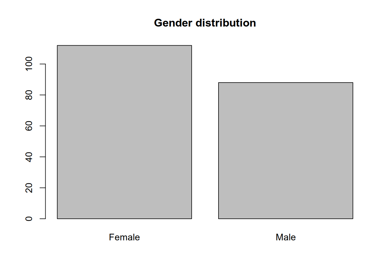

## The frequency table simply contains the number of male customers and the number of female customers

## Alternatively you can count the number of times "Female" occurs in the
## column "Gender" (see question j)

isFemale <- (mall$Gender == "Female")
sum(isFemale)

## [1] 112

12. Is there a difference (on average) between the age of female and male customers?

## In this task we need to compare 
## the average age of male and female customers

## First we create a logical vector that is TRUE
## if the customer is male and FALSE otherwise 

## First we compute the average age for male customers. Then 
## we use that vector to select only the age values of the male
## customers and finally we compute the mean of these values.

isMale <- mall$Gender == "Male"

## 
ageMaleCustomers <- mall$Age[isMale]

avgAgeMaleCustomers <- mean(ageMaleCustomers)

## Repeat the same for the female customers
## Note that "!" negates a logical vector. This works
## because we have only two categories Male/Female

ageFemaleCustomers <- mall$Age[!isMale]
avgAgeFemaleCustomers <- mean(ageFemaleCustomers)


## The average age of female customers is: 38.09
## The average age of male customers is: 39.8
## The female customers were therefore
avgAgeFemaleCustomers - avgAgeMaleCustomers

## [1] -1.708604

## years years younger (on average) than the male customers.

13. Use a box plot to compare the distribution of age by gender.

## Often it is quite useful to compare the distribution 
## of a variable between groups.
## The boxplot is one of the most important
## data displays for this task

## Here we create a boxplot for the distribution of age
## between male and female customers

boxplot(Age ~ Gender, data = mall, horizontal = TRUE)
title('Boxplot for Age by Gender')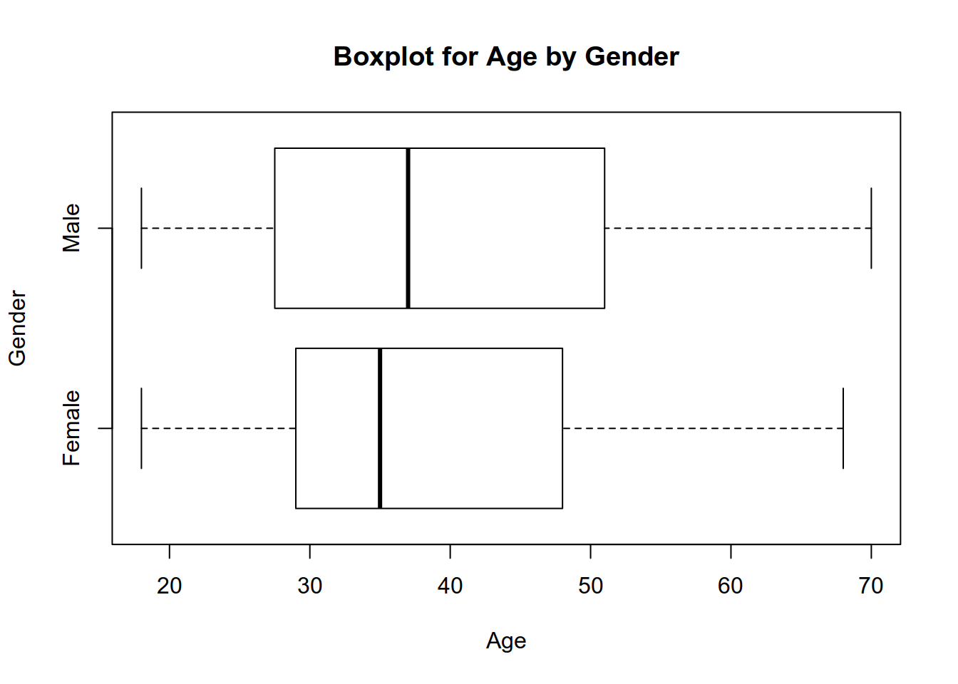

## The boxplot displays the median (thick line in the middle)
## and hinges (roughly corresponding to the first and third quartiles)
## For more on boxplots and how to interpret these, refer to Heumann et al (2015), p. 56

14. Use a scatter plot to examine how Score varies with age. Interpret the result.

## In the following assume that the score column contains a measurement of purchasing propensity
## of the customers (i.e. customers with higher score tend to spend more on purchases in the mall and
## customers with a low score tend to spend less in the mall)

## In this task we would like to create a scatterplot of Age and Score to examine the
## association pattern between the two variables

plot(mall$Age, mall$Score, xlab = "Age (years)", ylab = "Score")
title('Score and age plot')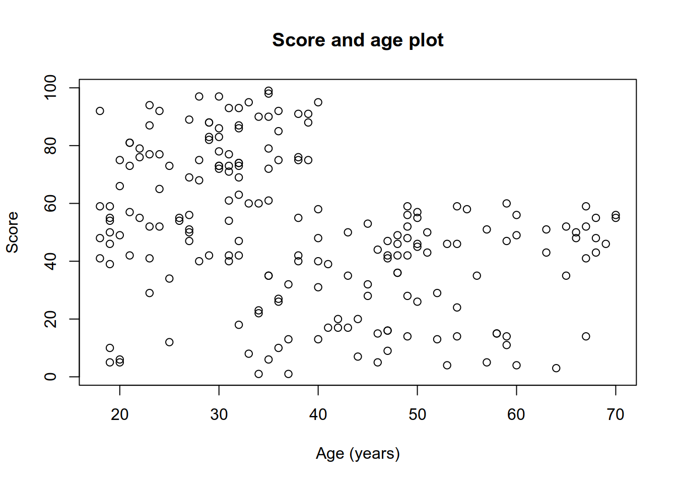

## Interpretation: the scatter plot indicates
## that customers over 40 years of age tend to 
## spend less (lower average score) than
## younger customers (18 - 40 years old)

9.2 Assignment 2 (Linear regression 1)

You can find the code for this exercise here. A detailed discussion of the methods used here is available in Chapter 8.1.

Disclaimer: As in the previous homework, please note that the dataset used here is simplified for ease of use and the analysis here MUST be viewed as an exercise, not real-world research! For the full dataset always refer to the data source!

The dataset linton is an adapted version of the data Linton et al. (2020) use to study the incubation period of SARS-CoV-19, the virus that causes COVID19. It contains 114 observations on COVID19 patients, mainly from mainland China. For this homework we are only interested in the variable Incubation
that measures the time in days from exposure to the virus to symptoms onset.

Before you begin you may find the following source useful:

• Simple regression model: Heumann and Shalabh (2016), pp. 249-259.
• Hypothesis testing: Heumann and Shalabh (2016), pp. 219-221.
• Confidence interval: Heumann and Shalabh (2016), pp. 197-199.
• Normal distribution: Heumann and Shalabh (2016), pp. 166-169.

1. Read and download the data (already done in the starter code)
2. Let \(y_i\) denote the incubation time for patient \(i = 1,\ldots,n\). Let \(u_i \sim N(0, \sigma ^ 2)\) be a normally distributed random variable with zero mean and variance \(\sigma ^ 2\). Furthermore, assume that the error terms \(u_i\) are independent. Fit the linear regression model:

\[\begin{align} y_i = \beta_0 + u_i, \quad i = 1,\ldots,n. \tag{9.1} \end{align}\]

Hint: use the lm function in R.

  fit <- lm(Incubation ~ 1, data = linton) ## This instructs lm to use only a constant

2. Print the summary of the regression fit

  summary(fit)

3. Write down the estimated regression equation (as a comment in the code).

4. What is the meaning of the intercept \(\beta_0\) in the model? Write your answer in plain language as a comment in the code.

5. Given the hypothesis:

\[\begin{align} H_0: \beta_0 = 8 \tag{9.2}\\ H_1: \beta_0 \neq 8 \tag{9.3} \end{align}\]

• Explain the meaning of (9.2) in plain language.
  • Using the regression output, test the hypothesis at a 5 percent significance level and write down your decision to reject or not to reject the null hypothesis.

5. Estimate a 95 percent confidence interval for \(\beta_0\).

6. Using the regression output, estimate the probability that a randomly chosen person will have an incubation period between 5 and 10 days.

7. Do you see any problems with the choice of the statistical model in (9.1)?

First we download and read the data.

linton <- read.csv('https://firebasestorage.googleapis.com/v0/b/uni-sofia.appspot.com/o/data%2Flinton2020_complete_obs.csv?alt=media&token=1ba3e0d4-658b-4639-ae5b-408e9e109047', stringsAsFactors = FALSE)

Next we estimate the regression model: \[\begin{align*} y_i = \beta_0 + u_i, \quad u_i \sim N(0, \sigma ^ 2) \end{align*}\]

  fit <- lm(Incubation ~ 1, data = linton)

and print the result of the fit summary:

  summary(fit)

## 
## Call:
## lm(formula = Incubation ~ 1, data = linton)
## 
## Residuals:
##     Min      1Q  Median      3Q     Max 
## -3.8947 -2.3947 -1.3947  0.6053 19.1053 
## 
## Coefficients:
##             Estimate Std. Error t value Pr(>|t|)    
## (Intercept)   5.3947     0.4247    12.7   <2e-16 ***
## ---
## Signif. codes:  0 '***' 0.001 '**' 0.01 '*' 0.05 '.' 0.1 ' ' 1
## 
## Residual standard error: 4.534 on 113 degrees of freedom

The estimated regression equation is \[\begin{align} \hat{y} = \hat{\beta_0}. \tag{8.8} \end{align}\] Inserting the estimate for \(\beta_0\) (look at the regression summary) into (8.8) we obtain \[\begin{align} \hat{y} = 5.39. \end{align}\]

9.3 Assignment 3 (Linear regression, 0/1 predictor)

9.3.1 English

In the current assignment we will take a break from the coronavirus examples and will focus on a study of intelligence in kids. The dataset kids is a subsample of the National Longitudinal Survey of Youth, USA, and contains measurements of cognitive test scores of three- and four- year-old children. Furthermore, it contains data on the education background of the kids’ mothers.

• kid_score: (numeric) Kid’s IQ score.
• mom_hs (binary): 1 if the mother has finished high school, 0 otherwise.

1. Download and read the dataset into an object called kids.

kids <- read.csv("https://raw.githubusercontent.com/feb-uni-sofia/econometrics2020-solutions/master/data/childiq.csv", stringsAsFactors = FALSE)
str(kids)

## 'data.frame':    434 obs. of  5 variables:
##  $ kid_score: int  65 98 85 83 115 98 69 106 102 95 ...
##  $ mom_hs   : int  1 1 1 1 1 0 1 1 1 1 ...
##  $ mom_iq   : num  121.1 89.4 115.4 99.4 92.7 ...
##  $ mom_work : int  4 4 4 3 4 1 4 3 1 1 ...
##  $ mom_age  : int  27 25 27 25 27 18 20 23 24 19 ...

2. Compute the average IQ score of children whose mother has not completed her high school education [mom_hs == 0] and compare it with the average IQ score of children whose mother has a high school degree [mom_hs == 1].

mean(kids$kid_score)

## [1] 86.79724

## Average IQ of kids where the mother has no HS degree
mean(kids$kid_score[kids$mom_hs == 0])

## [1] 77.54839

## Average IQ of kids where the mother has graduated HS
mean(kids$kid_score[kids$mom_hs == 1])

## [1] 89.31965

## Or alternatively using the dplyr package
## Run 
## install.packages("dplyr")
## on your system before loading the package. You only need to install a package once (per computer).

library(dplyr)

kids %>%
  group_by(mom_hs) %>%
  summarise(
    avgIQ = mean(kid_score)
  )

## # A tibble: 2 x 2
##   mom_hs avgIQ
##    <int> <dbl>
## 1      0  77.5
## 2      1  89.3

4. Create a scatter plot of kid_score and mom_hs. Draw the estimated regression line (use abline). Use the jitter function for the values of mom_hs to avoid overplotting.

plot(
  y = kids$kid_score, 
  x = jitter(kids$mom_hs, 0.2), 
  xlab="Mother has high school education.", 
  ylab = "IQ test score",
  main="IQ scores by mother's education status."
  )
abline(a = 77.548, b = 11.771, lty = 2)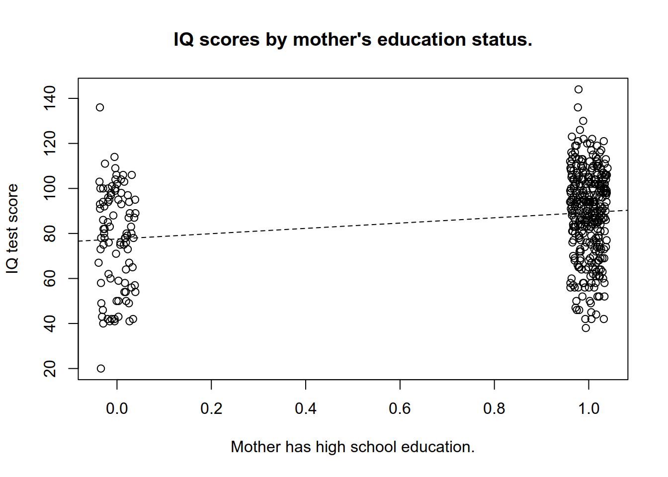

3. Let \(i=1,\ldots,n\) index the children observed in the sample. Let \(x_i\) denote the IQ score of the \(i\)-th kid and let \(x_i \in \{0, 1\}\) denote the high school status of the mother of the \(i-th\) kid. Fit the linear regression model:

\[ y_i = \beta_0 + \beta_1 x_i + u_i, \quad u_i \sim N(0, \sigma ^2) \]

Assume that \(u_i\) are independent and normally distributed with \(N(0, \sigma ^ 2)\) for all \(i=1,\ldots,n\). Compute the OLS estimates \(\hat{\beta}_0\) and \(\hat{\beta}_1\) for the regression coefficients and write down the estimated regression equation regression line.

fit <- lm(kid_score ~ mom_hs, data = kids)
summary(fit)

## 
## Call:
## lm(formula = kid_score ~ mom_hs, data = kids)
## 
## Residuals:
##    Min     1Q Median     3Q    Max 
## -57.55 -13.32   2.68  14.68  58.45 
## 
## Coefficients:
##             Estimate Std. Error t value Pr(>|t|)    
## (Intercept)   77.548      2.059  37.670  < 2e-16 ***
## mom_hs        11.771      2.322   5.069 5.96e-07 ***
## ---
## Signif. codes:  0 '***' 0.001 '**' 0.01 '*' 0.05 '.' 0.1 ' ' 1
## 
## Residual standard error: 19.85 on 432 degrees of freedom
## Multiple R-squared:  0.05613,    Adjusted R-squared:  0.05394 
## F-statistic: 25.69 on 1 and 432 DF,  p-value: 5.957e-07

\[ y = \beta_0 + \beta_1 x + u, \quad u \sim N(0, \sigma ^2) \]

4. Let \(\mu_0 = E(y | x = 0)\) denote the expected IQ of kids with mothers without a high school degree. Let \(\mu_1 = E(y | x = 1)\) denote the expected IQ of kids with mothers who have graduated a high school. Express the hypothesis

\[\begin{align} H_0: \mu_0 & = \mu_1\\ H_1: \mu_1 & \neq \mu_0 \end{align}\]

To relate the null hypothesis to the model coefficients \(\beta_0, \beta_1\) compute the conditional expecation of \(y\) given \(x\).

\[ E(y|x) = E(\beta_0 + \beta_1 x + u | x) \\ E(y|x) = \beta_0 + E(\beta_1 x + u | x) \\ E(y|x) = \beta_0 + \beta_1 x + \underbrace{E( u | x)}_{ = 0 \text{ by assumption}} \\ E(y|x) = \beta_0 + \beta_1 x \] In this problem can only have two possible values: \(x \in \{0, 1\}\). Compute the expected value of \(y\) for \(x = 0\) and \(x = 1\) to obtain: \[ E(y|x = 0) = \beta_0 + \beta_1 \times 0\\ E(y|x = 1) = \beta_0 + \beta_1 \times 1\\ \] and rearrange the two equations so that you have \(\beta_0\) and \(\beta_1\) on the left hand side. \[ \beta_0 = E(y|x = 0) \\ \beta_1 = E(y|x = 1) - E(y|x = 0) \] From these two equations you obtain the meaning of the coefficients. \(\beta_0\) is the expected IQ score for children whose mothers had no high school eucation (\(x = 0\)). \(\beta_1\) is the difference between the expected IQ scores in the two groups.

Now you can express the null hypothesis in terms of the model coefficients:

\[ E(y|x = 1) = E(y|x = 0) \iff E(y|x = 1) - E(y|x = 0) = 0 \iff \beta_1 = 0 \] \[ H_0: \beta_1 = 0 \\ H_1: \beta_1 \neq 0 \] Use the t-test to test the hypothesis. The t-statistic is \[ T = \frac{\hat{\beta}_1 - \beta_1^{H_0}}{SE(\hat{\beta}_1)} \stackrel{H_0}{\sim} t(n - 2) \] and follows a \(t(n - 2)\) distribution under the null hypothesis. Note that the number of degrees of freedom is \(n - 2\). As a rule remember that for coefficient test the degrees of freedom equal the number of observations \(n\) minus the number of model coefficients \(p\). In the model there there are two coefficients: \(\beta_0\) and \(\beta_1\), so \(p = 2\). With the values of \(\hat{\beta}_1\) and \(SE(\hat{\beta}_1)\) from the lm output we can compute the t-statistic as follows: \[ t = \frac{11.771 - 0}{2.322} = 5.069337 \]

tStat <- (11.771 - 0) / 2.322
tStat

## [1] 5.069337

Then we can compute the critical values at the 5 percent significance level

lowerCritical <- qt(0.05 / 2, df = 434 - 2)
upperCritical <- - lowerCritical
lowerCritical

## [1] -1.965471

upperCritical

## [1] 1.965471

The t-statistic is less than the lower critical value, therefor we reject \(H_0\) at the 5 percent significance level. Alternatively we can compute the p-value of the test

\[\begin{align} p-value & = P(|T| > |t|) = P((T < -|t|) \cup (T > |t|)) = \\ & = P((T < -|t|) + P((T > |t|)) \end{align}\]

pt(-5.069337, df = 434 - 2)

## [1] 2.966166e-07

1 - pt(5.069337, df = 434 - 2)

## [1] 2.966166e-07

2 * pt(-5.069337, df = 434 - 2)

## [1] 5.932331e-07

We reject \(H_0\) because the p-value of the test equals 5.932331e-07 and is less 0.05 (significance level).

1. Test the following hypothesis pair:

\[ H_0: \beta_1 = 10 \\ H_0: \beta_1 \neq 10 \] \[ t = \frac{11.771 - 10}{2.322} = 0.76 \]

(11.771 - 10) / 2.322 

## [1] 0.7627046

pt(-0.76, df = 434 - 2) ## P(T < -0.76)

## [1] 0.2238346

1 - pt(0.76, df = 434 - 2) ## P(T > 0.76)

## [1] 0.2238346

2*pt(-0.76, df = 434 - 2) ## P(T < -0.76)

## [1] 0.4476691

We cannot reject \(H_0: \beta_1 = 10\) at the 5 percent significance level, because the p-value (0.44) is greater than 0.05.

9.3.2 Български

Наборът от данни kids е част от извадката на Национално Излседване на младежи National Longitudinal Survey of Youth (USA) и съръжда резултати от тестове за интелигентност на деца между 3 и 4 годишна възраст. Също така съдържа данни за завършено средно образование на майките на децата.

• kid_score: (numeric) Точки от теста за интелигентност.
• mom_hs (binary): 1: майката има завършено средно образование, 0: без завършено средно образование.

1. Прочетете данните и ги запишете в обект на име kids.

kids <- read.csv("https://raw.githubusercontent.com/feb-uni-sofia/econometrics2020-solutions/master/data/childiq.csv", stringsAsFactors = FALSE)
str(kids)

## 'data.frame':    434 obs. of  5 variables:
##  $ kid_score: int  65 98 85 83 115 98 69 106 102 95 ...
##  $ mom_hs   : int  1 1 1 1 1 0 1 1 1 1 ...
##  $ mom_iq   : num  121.1 89.4 115.4 99.4 92.7 ...
##  $ mom_work : int  4 4 4 3 4 1 4 3 1 1 ...
##  $ mom_age  : int  27 25 27 25 27 18 20 23 24 19 ...

2. Пресметнете средния коефициент на интелигентност на децата според статуса на майките им и сравнете средните стойност на двете групи деца.

## Среден IQ на деца с майка без средно образование
mean(kids$kid_score[kids$mom_hs == 0])

## [1] 77.54839

## Среден IQ на деца с майка със средно образование
mean(kids$kid_score[kids$mom_hs == 1])

## [1] 89.31965

## Друг начин за същото изчисление
## Инсталирайте пакета dplyr на компютъра
## install.packages("dplyr")
## преди да заредите пакета. Достатъчно е да изпълните install.packages("dplyr") веднъж.

library(dplyr)

kids %>%
  group_by(mom_hs) %>%
  summarise(
    avgIQ = mean(kid_score)
  )

## `summarise()` ungrouping output (override with `.groups` argument)

## # A tibble: 2 x 2
##   mom_hs avgIQ
##    <int> <dbl>
## 1      0  77.5
## 2      1  89.3

3. Нека означим с \(i=1,\ldots,n\) номера на всяко дете в извадката. Нека \(x_i\) означва точките от теста за интелигеност на дете \(i\) и нека \(x_i \in \{0, 1\}\) да означава статусът на майката на дете \(i\). Оценете : \[\begin{align} y_i = \beta_0 + x_i + u_i \end{align}\] Да допуснем, че \(u_i ~ N(0, \sigma ^ 2)\) за всяко \(i=1,\ldots,n\).

Изчислете оценките \(\hat{\beta}_0\) и \(\hat{\beta}_1\) за регресионните коефициенти като използвате метода на най-малките квадрати (OLS). Напишете оцененото регресионно уравнение.

4. Създайте scatter plot диаграма на kid_score и mom_hs. Начертайте оценената регресионна права. Използвайте функцията jitter за стойностите на mom_hs, за да избегнете струпване на точки една върху друга.

plot(
  y = kids$kid_score, 
  x = jitter(kids$mom_hs, 0.2), 
  xlab="Mother has high school education.", 
  ylab = "IQ test score",
  main="IQ scores by mother's education status.",
  )
abline(a = 77.548, b = 11.771, lty = 2)

4. Нека \(\mu_0 = E(y | x = 0)\) означава очакваната стойност на IQ на деца с майки, които нямат завършено средно образование. Нека \(\mu_1 = E(y | x = 1)\) означава очаквания IQ на деца, чиято майка е завършила средно образование. Изразете хипотезата

\[\begin{align} H_0: \mu_0 & = \mu_1\\ H_1: \mu_1 & \neq \mu_0 \end{align}\]

с коефициентите на модела \(\beta_0\) and \(\beta_1\) и тействайте хипотезата при ниво на сигнификантност \(\alpha = 0.05\).

9.4 Assignment 4 (Linear regression, one continuous predictor)

9.4.1 English

Suppose that you are hired to advise the manager of a purchasing department. The manager would like to estimate the average amount of time necessary to proccess a given number of invoices. You are given data collected over 30 days with two variables:

• Invoices: (numeric) Number of processed invoices.
• Time (numeric): Work time in hours needed to process the invoices.

1. Download and read the data

invoices <- read.delim('https://raw.githubusercontent.com/feb-uni-sofia/econometrics2020-solutions/master/data/invoices.txt')
str(invoices)

## 'data.frame':    30 obs. of  3 variables:
##  $ Day     : int  1 2 3 4 5 6 7 8 9 10 ...
##  $ Invoices: int  149 60 188 23 201 58 77 222 181 30 ...
##  $ Time    : num  2.1 1.8 2.3 0.8 2.7 1 1.7 3.1 2.8 1 ...

2. Create a scatterplot data and interpret the graphic.

plot(invoices$Invoices, invoices$Time, ylab = "Time (in hours)", xlab = "Number of invoices")

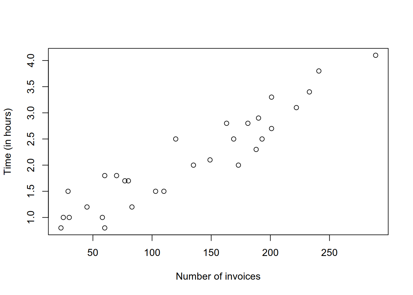
From the scatterplot you can see a pronounced linear association between the number of invoies and the work time in hours.

3. Let \(y\) denote the work time needed to process \(x\) invoices. Consider the model

\[ y_i = \beta_0 + \beta_1 x_i + u_i \]

\[\begin{align} y_i = \beta_0 + \beta_1 x_i + u_i \end{align}\] where \(u_i\) are independent and normally distributed with zero mean and variance \(\sigma^2\). What is the meaning of the coefficients \(\beta_0\) and \(\beta_1\) in this model? Explain using plain language.

To see how to interpret the coefficients, compute the conditional expectation of \(y\) given \(x\).

\[ E(y|x) = E(\beta_0 + \beta_1x + u | x) \\ E(y|x) = \beta_0 + \beta_1x + E(u | x), \quad E(u | x) = 0 \quad \text{by assumption} \\ E(y|x) = \beta_0 + \beta_1x \\ \] For \(x = 0\) this expectation is equal to \(\beta_0\)

\[ E(y|x = 0) = \beta_0 + \beta_1 \times 0 \\ E(y|x = 0)= \beta_0 \] The expected work time at zero number of invoices (\(x = 0\)) is \(\beta_0\). You can interpret this as the fixed (independent of the work load) costs of the firm in terms of time.

To interpret \(\beta_1\) look at the difference of the two expected values: \(E(y|x = x_0)\) and \(E(y|x = x_1)\).

\[ E(y|x = x_1) - E(y|x = x_0) = \beta_0 + \beta_1 x_1 - \beta_0 - \beta_1 x_1 \\ = \beta_1(x_1 - x_0) \\ \] Let \(x_1 - x_0 = 1\). You see that the expected value of \(y\) given \(x\) is \(\beta_1\) hours higher for one additional invoice.

\[ \widehat{E(y | x = 0)} = \hat{\beta} = 0.64\\ \frac{\partial\hat{y}}{\partial x} = 0.011\\ \widehat{E(y| x = 1)} - \widehat{E(y | x = 0)} = 0.011\\ \widehat{E(y| x = 101)} - \widehat{E(y | x = 51)} = (101 - 51) \times 0.011 \]

\[ \hat{y} = \widehat{E(y|x)} = \hat{\beta}_0 + \hat{\beta}_1x\\ \hat{\beta_0} = 0.64, \hat{\beta_1} = 0.011\\ \widehat{E(y|x)} = \hat{y} = 0.64 + 0.011x\\ \] Make sure that you understand the measurement unit of the coefficients. The measurement unit of the left-hand side of the equation must be the same as the measurement unit of the right-hand side. In this example \(y\) is measured in hours. Therefore \(\beta_0\) is also measured in hours. \(x\) is a number of invoices and \(\beta_1 \times x\) must be measured in hours, otherwise the equation would not make any sense. From there you see that \(\beta_1\) is measured in hours per invoice.

\[ hours = hours + \underbrace{\frac{hours}{\text{number of invoices}} \times [\text{number of invoices}]}_{\text{hours}} \]

4. Estimate \(\beta_0\), \(\beta_1\) and \(\sigma\) using OLS (lm function in R.). Store the fitted model in an object called fit. Plot the estimated regression line.

fit <- lm(Time ~ Invoices, data = invoices)
summary(fit)

## 
## Call:
## lm(formula = Time ~ Invoices, data = invoices)
## 
## Residuals:
##      Min       1Q   Median       3Q      Max 
## -0.59516 -0.27851  0.03485  0.19346  0.53083 
## 
## Coefficients:
##              Estimate Std. Error t value Pr(>|t|)    
## (Intercept) 0.6417099  0.1222707   5.248 1.41e-05 ***
## Invoices    0.0112916  0.0008184  13.797 5.17e-14 ***
## ---
## Signif. codes:  0 '***' 0.001 '**' 0.01 '*' 0.05 '.' 0.1 ' ' 1
## 
## Residual standard error: 0.3298 on 28 degrees of freedom
## Multiple R-squared:  0.8718, Adjusted R-squared:  0.8672 
## F-statistic: 190.4 on 1 and 28 DF,  p-value: 5.175e-14

plot(x = invoices$Invoices, y = invoices$Time)
abline(a = fit$coefficients[1], b = fit$coefficients[2])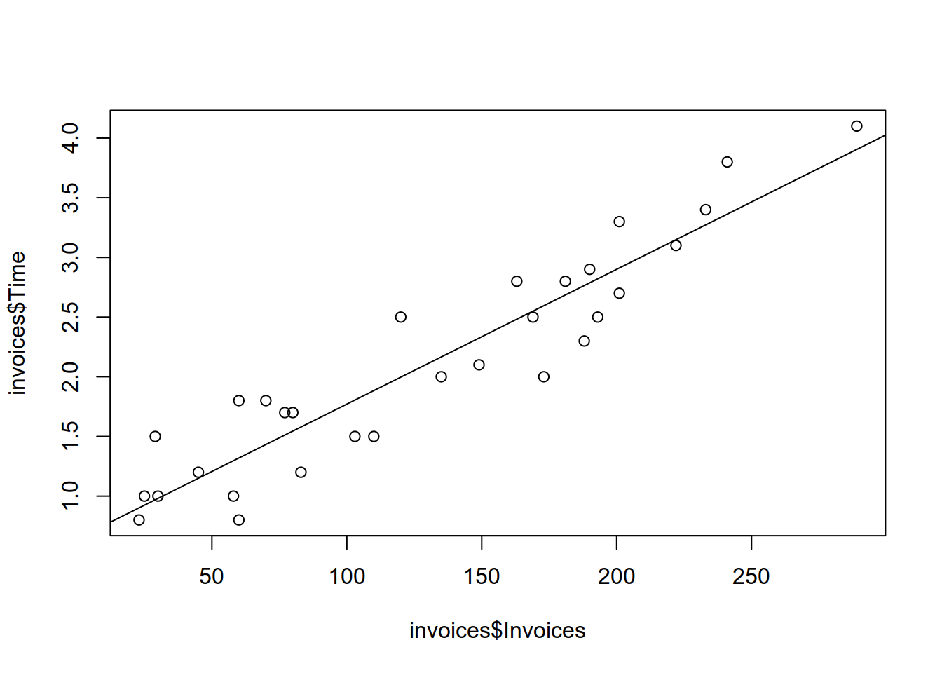

\[ \hat{y} = \widehat{E(y|x)} = \hat{\beta}_0 + \hat{\beta}_1x\\ \hat{\beta_0} = 0.64, \hat{\beta_1} = 0.011\\ \hat{y} = 0.64 + 0.011x \] 5. Estimate the expected time to process 130 invoices. Compute both a point and a 95 percent interval estimate using the output of summary(fit).

The expected time to process the 130 invoices is \[ E(y|x = 130) = \beta_0 + \beta_1\times 130 \] Both \(\beta_0\) and \(\beta_1\) are unknown so we cannot compute it directly. To estimate it, insert the estimated values of the model coefficients (see the output of lm).

\[ \widehat{E(y| x = 130)} = 0.64 + 0.011 \times 130 \] For the interval estimate of \(E(y|x = 130)\) we will use predict with the interval argument.

yhat130 <- predict(fit, newdata = data.frame(Invoices = 130), interval = "confidence", level = 0.95)
yhat130

##        fit      lwr      upr
## 1 2.109624 1.986293 2.232954

We estimate \(E(y|x = 130)\) to be between \(1.98\) and \(2.23\) hours (95 percent confidence interval).

6. Plot the estimated mean of \(y\) for 40 values between the lowest and the highest observed number of invoices.

xGrid <- seq(min(invoices$Invoices), max(invoices$Invoices), length.out = 40)
yhatConf <- predict(fit, newdata = data.frame(Invoices = xGrid), interval = "confidence", level = 0.95)
plot(x = invoices$Invoices, y = invoices$Time)
abline(a = fit$coefficients[1], b = fit$coefficients[2])
lines(xGrid, yhatConf[,2], col="blue", lty=2)
lines(xGrid, yhatConf[,3], col="blue", lty=2)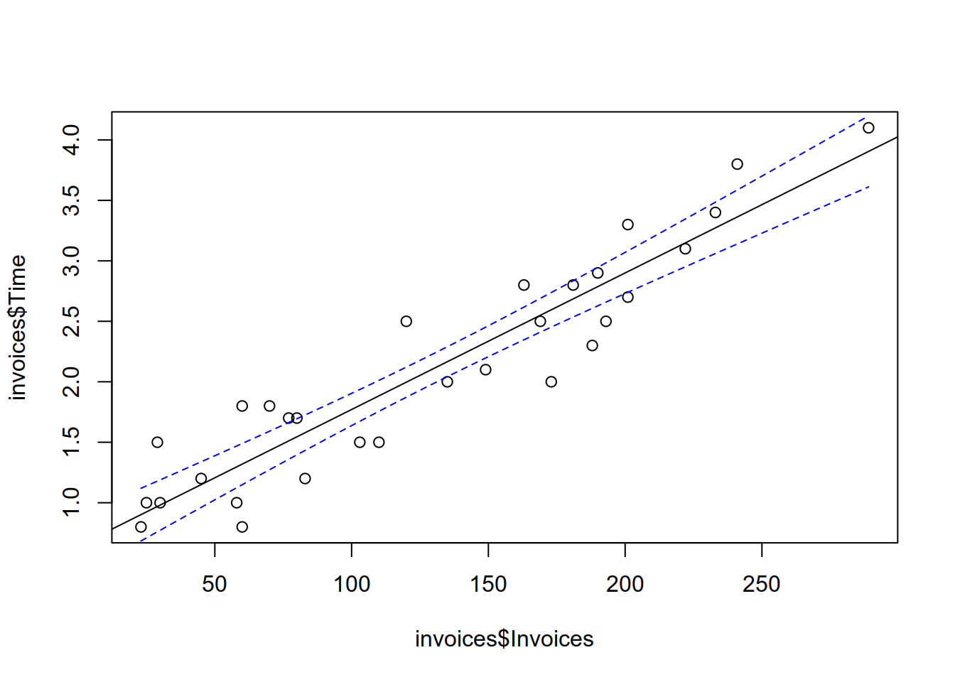

8. How much of the observed variation of Time is explained by Invoices?

The total observed variation (total sum of squares, SST) of \(y\) is defined as:

\[ \text{SST} = \sum_{i=1}^{n}(y_i - \bar{y})^2 \] It can be shown that we can decompose the total sum of squares into two other sums of squares called the regression sum of squares (SSReg) and residual sum of squares (RSS).

\[ \underbrace{\sum_{i=1}^{n}(y_i - \bar{y})^2}_{SST} = \underbrace{\sum_{i=1}^n(y_i - \hat{y}_i)^2}_{RSS} + \underbrace{\sum_{i=1}^n(\hat{y_i} - \bar{y})^2}_{SSReg} \] You can think of the two sums of squares on the right-hand side of the equation as variation explained by the model (SSReg) and variation not explained by the model (RSS). Now devide the equation by SST to obtain:

\[ 1 = \frac{RSS}{SST} + \frac{SSReg}{SST} \\ 1 - \frac{RSS}{SST} = \frac{SSReg}{SST} = R^2 \]

The ratio of SSReg and SST is called R^2 and you can interpret it as the share of variation of \(y\) that is explained by the model.

9. Explain the meaning of \(\beta_0\) in the following regression model:

\[\begin{align} y = \beta_0 + u_i \tag{9.4} \end{align}\]

In this model \(\beta_0\) is simply the expected work time per day:

\[ E(y) = \beta_0 \]

10. Plot the estimated regression line of (9.4).

plot(x = invoices$Invoices, y = invoices$Time)
abline(h = mean(invoices$Time))

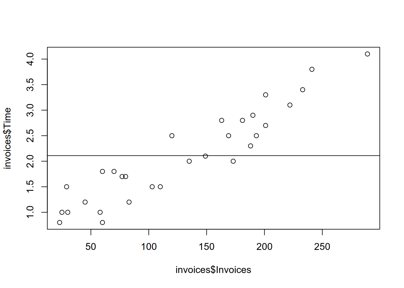
9.4.2 Български

Представете си, че управител на фирма ви е наел, за да анлизирате работата на счетоводния отдел на фирма. Част от работното време на този отдел е ангажирано с обработка на фактури, които постъпват във фирмата. В набора от данни invoices са записани броя фактури и времето им за обработка в продължение на 30 дена.

• Invoices: (numeric) Брой обработени фактури.
• Time (numeric): Време (в часове) за обработка на фактурите.

1. Прочетете данните.

invoices <- read.delim('https://raw.githubusercontent.com/feb-uni-sofia/econometrics2020-solutions/master/data/invoices.txt')
str(invoices)

## 'data.frame':    30 obs. of  3 variables:
##  $ Day     : int  1 2 3 4 5 6 7 8 9 10 ...
##  $ Invoices: int  149 60 188 23 201 58 77 222 181 30 ...
##  $ Time    : num  2.1 1.8 2.3 0.8 2.7 1 1.7 3.1 2.8 1 ...

2. Създайте scatterplot диаграма и интерпретирайте графиката.

plot(x = invoices$Invoices, y = invoices$Time)

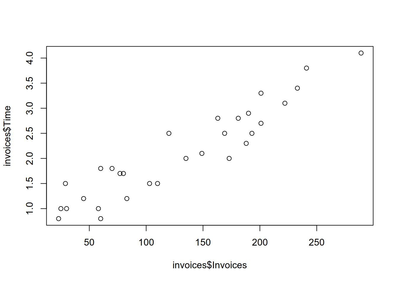3. Нека да означим с \(y\) работното време нужно за обработката на \(x\) фактури и да разгледаме следния линеен модел.

\[\begin{align} y_i = \beta_0 + \beta_1 x_i + u_i \tag{9.5} \end{align}\] Допуснете, че \(u_i\) са независими и нормално разпределени с очакване нула и дисперсия \(\sigma^2\). Какво е значението на коефициентите \(\beta_0\) и \(\beta_1\) в този модел?

За да интерпретираме коефициентите \(\beta_0\) и \(\beta_1\) първо ще изчислим условното очакване на \(y\) при даден \(x\).

\[ E(y|x) = \beta_0 + \beta_1 x \]

4. Оценете \(\beta_0\), \(\beta_1\) and \(\sigma\) с метода на най-малките квадрати (lm function in R.). Запишете резултата от lm в обект на име fit. Начертайте оценената регресионна права.

fit <- lm(Time ~ Invoices, data = invoices)
summary(fit)

## 
## Call:
## lm(formula = Time ~ Invoices, data = invoices)
## 
## Residuals:
##      Min       1Q   Median       3Q      Max 
## -0.59516 -0.27851  0.03485  0.19346  0.53083 
## 
## Coefficients:
##              Estimate Std. Error t value Pr(>|t|)    
## (Intercept) 0.6417099  0.1222707   5.248 1.41e-05 ***
## Invoices    0.0112916  0.0008184  13.797 5.17e-14 ***
## ---
## Signif. codes:  0 '***' 0.001 '**' 0.01 '*' 0.05 '.' 0.1 ' ' 1
## 
## Residual standard error: 0.3298 on 28 degrees of freedom
## Multiple R-squared:  0.8718, Adjusted R-squared:  0.8672 
## F-statistic: 190.4 on 1 and 28 DF,  p-value: 5.175e-14

5. Направете оценка за очакваното време за обработка на 130 фактури. Освен точкова оценка (point estimate) направете и 95 процентова интервална оценка като използвате summary(fit).

6. Използвайте фукцията predict с обекта, който съдържа оценения регресионен модел, за да направите същото изчисление като в предходния въпрос. В допълнение направете оценка за очакваното време за обработка за всяка наблюдавана стойност на \(x\).

predict(fit, newdata = data.frame(Invoices = 130))

##        1 
## 2.109624

predict(fit)

##         1         2         3         4         5         6         7         8 
## 2.3241648 1.3192085 2.7645390 0.9014177 2.9113303 1.2966252 1.5111665 3.1484549 
##         9        10        11        12        13        14        15        16 
## 2.6854975 0.9804592 1.8837907 1.5789163 1.3192085 0.9240010 2.5951643 2.5499977 
##        17        18        19        20        21        22        23        24 
## 2.7871223 3.2726630 3.9049950 1.1498339 2.8209972 1.4321250 3.3629961 1.8047492 
##        25        26        27        28        29        30 
## 2.4822479 1.9967072 2.9113303 2.1660818 1.5450414 0.9691676

predict(fit, newdata = data.frame(Invoices = 130), se.fit = TRUE, interval = c("confidence"), level = 0.95)

## $fit
##        fit      lwr      upr
## 1 2.109624 1.986293 2.232954
## 
## $se.fit
## [1] 0.0602081
## 
## $df
## [1] 28
## 
## $residual.scale
## [1] 0.3297733

predict(fit, newdata = data.frame(Invoices = 130), se.fit = TRUE, interval = "prediction", level = 0.95)

## $fit
##        fit      lwr    upr
## 1 2.109624 1.422947 2.7963
## 
## $se.fit
## [1] 0.0602081
## 
## $df
## [1] 28
## 
## $residual.scale
## [1] 0.3297733

2.109624 - qt(0.05 / 2, df = 28)  * sqrt(0.3297733 ^ 2 + 0.0602081 ^ 2)

## [1] 2.7963

qt(0.05 / 2, df = 28)

## [1] -2.048407

7. Управителят на фирмата твърди, че средното време за обработка на всяка допълнителна фактура е равно на 6 минути. Изразете твърдението на управителя с коефициентите на модел (9.5) и тествайте хипотезата (двустранно) при ниво на сигнификантност \(\alpha = 0.05\).

8. Каква част от вариацията на Time е обяснена с вариация на Invoices в модел (9.5)?

9. Обяснете значението на \(\beta_0\) в следния линеен модел:

\[\begin{align} y = \beta_0 + u_i \tag{9.6} \end{align}\]

10. Начертайте оценената регресионна права в модел (9.6).

9.5 Assignment 5: Multiple regression

The dataset crime contains data on crime rates in 67 counties in Florida, US.

County (character): County name C (numeric): Number of crimes per 1,000 persons I (numeric): Median income in the county HS (numeric): Share of persons with completed high school education U (numeric): Share of persons living in an urban environment.

1. Download and read the data

crime <- read.delim("https://raw.githubusercontent.com/feb-uni-sofia/econometrics2020-solutions/master/data/crime.csv", stringsAsFactors = FALSE)
str(crime)

## 'data.frame':    67 obs. of  5 variables:
##  $ County: chr  "ALACHUA" "BAKER" "BAY" "BRADFORD" ...
##  $ C     : int  104 20 64 50 64 94 8 35 27 41 ...
##  $ I     : num  22.1 25.8 24.7 24.6 30.5 30.6 18.6 25.7 21.3 34.9 ...
##  $ HS    : num  82.7 64.1 74.7 65 82.3 76.8 55.9 75.7 68.6 81.2 ...
##  $ U     : num  73.2 21.5 85 23.2 91.9 98.9 0 80.2 31 65.8 ...

1. Create a scatterplot matrix with the variables C,U,HS and I.

pairs(crime[, -1])

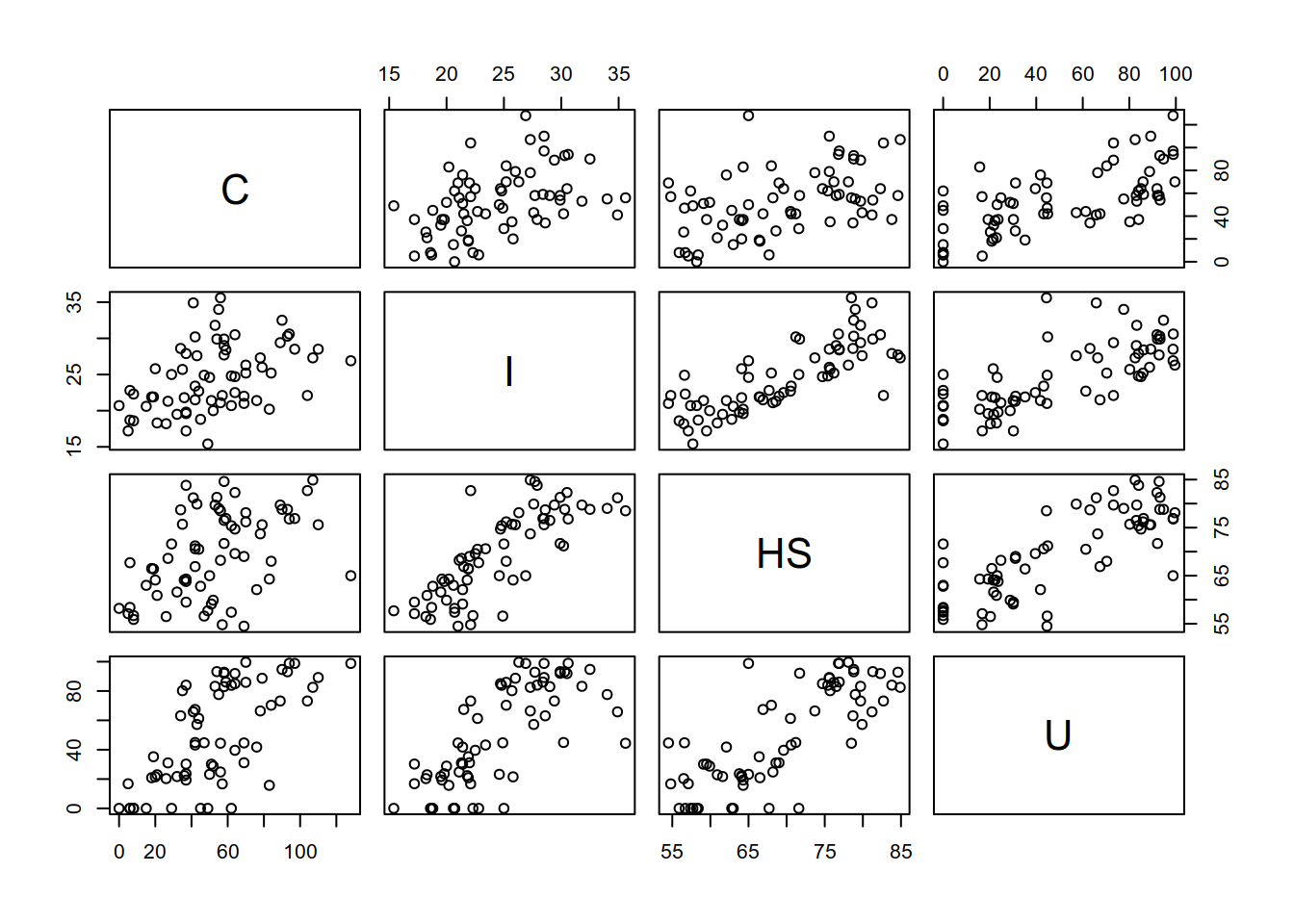
2. Fit the linear regression model. \[\begin{align} C_i = \beta_0+ \beta_1 HS_i + u_i \tag{9.7} \end{align}\] and interpret the estimated coefficients. Assume that \(u_i\) are independent random terms with variance \(\sigma^2\).

fitHS <- lm(C ~ HS, data = crime)
summary(fitHS)

## 
## Call:
## lm(formula = C ~ HS, data = crime)
## 
## Residuals:
##    Min     1Q Median     3Q    Max 
## -43.74 -21.36  -4.82  17.42  82.27 
## 
## Coefficients:
##             Estimate Std. Error t value Pr(>|t|)    
## (Intercept) -50.8569    24.4507  -2.080   0.0415 *  
## HS            1.4860     0.3491   4.257 6.81e-05 ***
## ---
## Signif. codes:  0 '***' 0.001 '**' 0.01 '*' 0.05 '.' 0.1 ' ' 1
## 
## Residual standard error: 25.12 on 65 degrees of freedom
## Multiple R-squared:  0.218,  Adjusted R-squared:  0.206 
## F-statistic: 18.12 on 1 and 65 DF,  p-value: 6.806e-05

To interpret the model coefficients, look at the conditional mean of \(C\) given \(HS\) \[ E(C|HS) = \beta_0 + \beta_1 HS \] \(\beta_0\) is the expected crime rate for a county that has no high school graduates at all.

\[ E(C|HS = 0) = \beta_0 + \beta_1 \times 0 = \beta_0 \]

The estimate for \(\beta_0\) is negative which does not make any sense as the crime rate must be non-negative. Look at the plot of the data (scatterplot matrix) and you should notice that the range of observed values of \(HS\) is far away from zero. Therefore, the intercept estimates the expected crime rate for a county that is quite different from the observed ones (extrapolation). Furthermore, our model imposes a strict (linear) relationship between HS and the expected crime rate.

\(\beta_1\) gives the difference of expected crime rates between two counties that differ by one percentage point on HS, e.g. 

\[ E(C|HS = 80) - E(C|HS = 79) = \beta_1 \]

The estimate for \(\beta_1\) is positive, which is surprising. This implies that counties with a higher share of high school graduates had (on average) a higher crime rate.

4. Fit the linear regression model \[\begin{align} C_i = \beta_0 + \beta_1 HS_i + \beta_2 U_i + u_i \tag{9.8} \end{align}\] and interpret the coefficients.

fitHS.U <- lm(C ~ HS + U, data = crime)
summary(fitHS.U)

## 
## Call:
## lm(formula = C ~ HS + U, data = crime)
## 
## Residuals:
##     Min      1Q  Median      3Q     Max 
## -34.693 -15.742  -6.226  15.812  50.678 
## 
## Coefficients:
##             Estimate Std. Error t value Pr(>|t|)    
## (Intercept)  59.1181    28.3653   2.084   0.0411 *  
## HS           -0.5834     0.4725  -1.235   0.2214    
## U             0.6825     0.1232   5.539 6.11e-07 ***
## ---
## Signif. codes:  0 '***' 0.001 '**' 0.01 '*' 0.05 '.' 0.1 ' ' 1
## 
## Residual standard error: 20.82 on 64 degrees of freedom
## Multiple R-squared:  0.4714, Adjusted R-squared:  0.4549 
## F-statistic: 28.54 on 2 and 64 DF,  p-value: 1.379e-09

Again as in the previous question, look at the expected crime rate in this model:

\[ E(C|HS, U) = \beta_0 + \beta_1 HS + \beta_2 U \] The intercept (\(\beta_0\)) is the expected crime rate that is entirely rural (Urbanicity = 0) and has no high school graduates (HS = 0).

\[ E(C|HS=0, U=0) = \beta_0 + \beta_1 \times 0 + \beta_2 \times 0 = \beta_0 \] \(\beta_1\) gives the difference between the expected crime rates of counties that differ by 1 percentage point on HS and have the same percentage of persons living in urban areas (U).

\[ E(C|HS = 80, U) - E(C|HS = 79, U) = \beta_0 + \beta_1 \times 80 + \beta_2 U - (\beta_0 + \beta_1 \times 79 + \beta_2 U) = \\ (80 - 79) \beta_1 = \beta_1 \] The coefficient \(\beta_2\) gives the difference between expected crime rates of counties that differn by 1 unit of U and have the same share of high school graduates (HS).

\[ E(C|HS, U = 50) - E(C|HS, U = 49) = \beta_0 + \beta_1 HS + \beta_2 \times 50 - (\beta_0 + \beta_1 HS + \beta_2 \times 49) = \beta_2 \] The coefficient of \(HS\) in this model is negative. This means that the expected crime rate was lower in counties with a larger share of high school graduates given a constant share of urban dwellers (U). The coefficient of U is positive, meaning that the crime rate was higher (on average) in urbanized counties compared to rural counties (low value of U) given a constant share of high school graduates.

In order to understand why the coefficient of HS is (radically) different in the two models discussed so far, look at the plot of the data. There you should notice that urbanicity (U) and the share of high school graduates (HS) are stronly (positively) correlated, meaning that educated persons (high school education) tend to live in urban areas. Because the crime rate tends to be higher in urban areas (again, look at the plot), our first model estimated a positive coefficint for HS.

The second model takes both HS and U into account. Controlling for the level of urbanization (i.e. holding U constant) we see that the relationship between education (HS) and the crime rate is negative.

5. Estimate the crime rate for a county where 80 percent of the polulation lives inurban areas and where 60 percent of the population has completed high school. Give approximate 95% prediction and confidence intervals.

Using the estimated regression equations \[ \widehat{E(C|HS, U)} = \hat{\beta}_0 + \hat{\beta}_1 HS + 0.6825 U \\ \implies \widehat{E(C|HS = 60, U = 80)} = \hat{\beta}_0 + \hat{\beta}_1 \times 60 + 0.6825 \times 80 = 78.71554 \] We can calculate the same entity using the predict function in R:

predict(fitHS.U, newdata = data.frame(HS = 60, U = 80))

##        1 
## 78.71554

We estimate the expected crime rate for a county with \(HS = 60\) and \(U = 80\) to be \(78.7\) per thousand persons.

\[ \widehat{E(C|HS, U)} = 59.1181 -0.5834 HS + \hat{\beta}_2 U \]

6. Fit the linear regression model

\[\begin{align} C_i =\beta_0 + \beta_1 HS_i + \beta_2 U_i + \beta_3 I_i + u_i \tag{9.9} \end{align}\]

and interpret the coefficients.

fitHS.U.I <- lm(C ~ HS + U + I, data = crime)
summary(fitHS.U.I)

## 
## Call:
## lm(formula = C ~ HS + U + I, data = crime)
## 
## Residuals:
##     Min      1Q  Median      3Q     Max 
## -35.407 -15.080  -6.588  16.178  50.125 
## 
## Coefficients:
##             Estimate Std. Error t value Pr(>|t|)    
## (Intercept)  59.7147    28.5895   2.089   0.0408 *  
## HS           -0.4673     0.5544  -0.843   0.4025    
## U             0.6972     0.1291   5.399 1.08e-06 ***
## I            -0.3831     0.9405  -0.407   0.6852    
## ---
## Signif. codes:  0 '***' 0.001 '**' 0.01 '*' 0.05 '.' 0.1 ' ' 1
## 
## Residual standard error: 20.95 on 63 degrees of freedom
## Multiple R-squared:  0.4728, Adjusted R-squared:  0.4477 
## F-statistic: 18.83 on 3 and 63 DF,  p-value: 7.823e-09

7. Compare the model from (9.9) with the reduced model: \(C_i=\beta_0 \beta_1 U_i + u_i\). Which model would you prefer for explaining the variation of crime rates?

fitU <- lm(C ~ U, data = crime)

anova(fitU, fitHS.U.I)

## Analysis of Variance Table
## 
## Model 1: C ~ U
## Model 2: C ~ HS + U + I
##   Res.Df   RSS Df Sum of Sq      F Pr(>F)
## 1     65 28391                           
## 2     63 27658  2    733.45 0.8353 0.4385

9.6 Assignment 6 (Linear regression, 0/1 and continuous predictors)

9.6.1 English

In the current assignment we will revisit the National Longitudinal Survey of Youth, USA and the kids dataset that contains measurements of cognitive test scores of three- and four- year-old children. Furthermore, it contains data on the education background of the kids’ mothers.

• kid_score: (numeric) Kid’s IQ score.
• mom_hs (binary): 1 if the mother has finished high school, 0 otherwise.
• mom_age (numeric): The age of the mother in years.
• mom_iq (numeric): The IQ score of the mother.

1. Download and read the dataset into an object called kids.

kids <- read.csv("https://raw.githubusercontent.com/feb-uni-sofia/econometrics2020-solutions/master/data/childiq.csv", stringsAsFactors = FALSE)
str(kids)

## 'data.frame':    434 obs. of  5 variables:
##  $ kid_score: int  65 98 85 83 115 98 69 106 102 95 ...
##  $ mom_hs   : int  1 1 1 1 1 0 1 1 1 1 ...
##  $ mom_iq   : num  121.1 89.4 115.4 99.4 92.7 ...
##  $ mom_work : int  4 4 4 3 4 1 4 3 1 1 ...
##  $ mom_age  : int  27 25 27 25 27 18 20 23 24 19 ...

fit <- lm(kid_score ~ mom_hs + mom_iq + mom_age, data = kids)
summary(fit)

## 
## Call:
## lm(formula = kid_score ~ mom_hs + mom_iq + mom_age, data = kids)
## 
## Residuals:
##     Min      1Q  Median      3Q     Max 
## -53.289 -12.421   2.399  11.223  50.169 
## 
## Coefficients:
##             Estimate Std. Error t value Pr(>|t|)    
## (Intercept) 20.98466    9.13013   2.298   0.0220 *  
## mom_hs       5.64715    2.25766   2.501   0.0127 *  
## mom_iq       0.56254    0.06065   9.276   <2e-16 ***
## mom_age      0.22475    0.33075   0.680   0.4972    
## ---
## Signif. codes:  0 '***' 0.001 '**' 0.01 '*' 0.05 '.' 0.1 ' ' 1
## 
## Residual standard error: 18.15 on 430 degrees of freedom
## Multiple R-squared:  0.215,  Adjusted R-squared:  0.2095 
## F-statistic: 39.25 on 3 and 430 DF,  p-value: < 2.2e-16

9.7 Test Exam (EN)

Github classroom link: https://classroom.github.com/a/6qyOBByc

9.7.1 Problem 1

The importance of academic performance is expected to increase in the next decades because of advances in new technologies and a shift of economic activities away from manual labour to knowledge-intensive labor. In this problem you will be modelling the academic performance of students (school children). The dataset students contains the following data on 1000 students. You will be working with a 300 observations subset of this data set.

[math.score] (numeric): Score from math problems (0 - 100). [reading.score] (numeric): Score from reading problems (0 - 100).

1. Download and read the dataset.

students <- read.csv("https://raw.githubusercontent.com/feb-uni-sofia/econometrics2020-solutions/master/data/StudentsPerformance.csv", stringsAsFactors = FALSE)

1. Create a new variable in the dataset students called math.score.centered that equals math.score minus the average math score.

students$math.score.centered <- students$math.score - mean(students$math.score)

2. Fit the linear regression model: \[\begin{align} \text{reading.score}_i = \beta_0 + \beta_1 \text{math.score.centered}_i + u_i \end{align}\] with \(i = 1,\ldots,n\) and where \(u_i\) are uncorrelated random terms with zero mean and constant variance.

fit <- lm(reading.score ~ math.score.centered, data = students)
summary(fit)

## 
## Call:
## lm(formula = reading.score ~ math.score.centered, data = students)
## 
## Residuals:
##      Min       1Q   Median       3Q      Max 
## -26.2905  -5.8011   0.1139   6.0341  21.4117 
## 
## Coefficients:
##                     Estimate Std. Error t value Pr(>|t|)    
## (Intercept)         69.16900    0.26599  260.05   <2e-16 ***
## math.score.centered  0.78723    0.01755   44.85   <2e-16 ***
## ---
## Signif. codes:  0 '***' 0.001 '**' 0.01 '*' 0.05 '.' 0.1 ' ' 1
## 
## Residual standard error: 8.411 on 998 degrees of freedom
## Multiple R-squared:  0.6684, Adjusted R-squared:  0.6681 
## F-statistic:  2012 on 1 and 998 DF,  p-value: < 2.2e-16

3. Write down the estimated regression equation. \[ \widehat{\text{reading.score}} = 69.16900 + 0.78723 \text{ math.score.centered} \]

4. What is the meaning of the intercept (\(\beta_0\)) in this model? This is the expected reading score for students who have achieve an average math score.

5. Interpret the sign of \(\hat{\beta_1}\). Does the estimated coefficient conform to your expectations? Explain why.

The sign of the coefficient for math score is positive. This implies that students with higher math score are expected to have higher average reading score.

6. Estimate the expected reading score for a student with average math score. Write down your estimate. Write down the standard error of this estimate and compute an approximate 95% prediction interval. Hint: use the predict function and write down your result: estimate and standard error.

predict(fit, newdata = data.frame(math.score.centered = 0), se.fit = TRUE, interval = "prediction")

## $fit
##      fit      lwr      upr
## 1 69.169 52.65503 85.68297
## 
## $se.fit
## [1] 0.2659864
## 
## $df
## [1] 998
## 
## $residual.scale
## [1] 8.411228

8. A teacher at the school claims that reading scores do not vary with differences in math score. Formulate a hypothesis (and an alternative) in terms of the model coefficients. Explain your decision to reject or not to reject the null hypothesis at a 5% significance level.

\[ H_0: \beta_1 = 0\\ H_1: \beta_1 \neq 0 \]

We can reject this hypothesis based on the p-value of the test, because \[2e-16 < 0.05\]

9.7.2 Problem 2

Bike sharing systems are a means of renting bicycles where the process of obtaining membership, rental, and bike return is automated via a network of kiosk locations throughout a city. In this problem you will be modelling the rental demand for bikes in Washington, D.C using historical usage patterns and weather data. The data set bikes contains observations on 10,886 hours of bike sharing service. You will be working with a 5000 observations subset of this data set.

[count] (numeric): Number of total bike rentals. [workingday] (numeric): 1: yes, 0: no.

1. Download and read the dataset.

bikes <- read.csv("https://raw.githubusercontent.com/feb-uni-sofia/econometrics2020-solutions/master/data/bikes.csv", stringsAsFactors = FALSE)

1. What is the average number of rentals per hour?

mean(bikes$count)

## [1] 191.5741

2. Create a new (logical) variable in the data.frame bikes called isWorkingday that equals TRUE if workingday equals 1 and that is FALSE otherwise.

bikes$isWorkingday <- (bikes$workingday == 1)

3. How many of the hours were recorded during the working days? (Write your answer below)

table(bikes$isWorkingday)

## 
## FALSE  TRUE 
##  3474  7412

4. Estimate the linear regression model:

\[\begin{align*} \text{count}_i = \beta_0 + \beta_1 \text{isWorkingday}_i + u_i \end{align*}\]

where \(u_i\), \(i = 1,\ldots,n\) are uncorrelated random terms with zero mean and constant variance. Write down the estimated regression equation.

fit <- lm(count ~ isWorkingday, data = bikes)
summary(fit)

## 
## Call:
## lm(formula = count ~ isWorkingday, data = bikes)
## 
## Residuals:
##     Min      1Q  Median      3Q     Max 
## -192.01 -148.89  -46.76   91.86  783.99 
## 
## Coefficients:
##                  Estimate Std. Error t value Pr(>|t|)    
## (Intercept)       188.507      3.073   61.34   <2e-16 ***
## isWorkingdayTRUE    4.505      3.724    1.21    0.226    
## ---
## Signif. codes:  0 '***' 0.001 '**' 0.01 '*' 0.05 '.' 0.1 ' ' 1
## 
## Residual standard error: 181.1 on 10884 degrees of freedom
## Multiple R-squared:  0.0001344,  Adjusted R-squared:  4.255e-05 
## F-statistic: 1.463 on 1 and 10884 DF,  p-value: 0.2264

5. Does the estimate of \(\beta_1\) conform to your expectations? Give a short explanation. The coefficient is positive, meaning that bikes were rented slightly more during work days, possibly because some people use these bikes to travel to their workplaces. During work the company rented 4.5 more bikes per hour on average compared to non-working days.

6. An employee at the bike sharing platform claims that there is no difference between the average number of rentals during work days and other days. Formulate a hypothesis (and an alternative) in terms of the model coefficients, compute and write down the value of the test-statistic and the p-value of the test. Explain your decision to reject or to not reject the hypothesis at the 5 percent significance level. (Your calculations need to be reproducible!) \[ H_0: \beta_1 = 0\\ H_1: \beta_1 \neq 0 \] Based on the p-value of the test we cannot reject this hypothesis, because it is larger than 0.05: \(0.26 > 0.05\).

7. Another employee claims that the average number of rentals during non-working days hours equals 220. Formulate her hypothesis in terms of the model coefficients, compute and write down the value of the test-statistic, the critical values at a 95% significance level (5% error probability). Explain your decision to reject or to not reject the hypothesis at the 95% significance level. Hint: use the qt function to calculate the critical values. \[ H_0: \beta_0 = 220 \\ H_1: \beta_0 \neq 220 \]

tStat <- (188.507 - 220) / 3.073
tStat

## [1] -10.24829

lowerCriticalValue <- qt(0.05 / 2, df = nrow(bikes) - 2)
lowerCriticalValue

## [1] -1.960182

We reject the null hypothesis at a 5 percent significance level, because the t-statistic is less than the lower critical value.

8. The manager of the bike sharing platform is curious about the meaning of the 5% error probability used in the test above. Give a short explanation.

9.8 Test Exam (BG)

Github classroom link: https://classroom.github.com/a/6qyOBByc

9.8.1 Задача 1 (Problem 1)

В тази задача целта е да се формулира модел, който описва академичните способности на ученици. Таблицата с данни students съдържа наблюдения върху 1000 ученика и следните характеристики (variables).

[math.score] (numeric): Брой точки от задачи по математика (0 - 100). [reading.score] (numeric): Брой точки от задачи по четене (0 - 100).

1. Прочетете изходните данни.

students <- read.csv("https://raw.githubusercontent.com/feb-uni-sofia/econometrics2020-solutions/master/data/StudentsPerformance.csv", stringsAsFactors = FALSE)

1. Създайте нова променлива в таблицата students на име math.score.centered която да е равна на math.score минус средната стойност на math.score.

2. Оценете регресионния модел \[\begin{align} \text{reading.score}_i = \beta_0 + \beta_1 \text{math.score.centered}_i + u_i \end{align}\] където \(i = 1,\ldots,n\) и \(u_i\) са независими нормално разпределени случайни грешки със средна стойност нула и дисперсия \(\sigma^2\).

3. Напишете оцененото регресионно уравнение.

4. Какво е значението на константата (\(\beta_0\)) в този модел?

5. Интерпретирайте знака на \(\hat{\beta_1}\). Получената оценка отговаря ли на вашите очаквания? Обяснете защо.

6. Направете оценка за очаквания брой точки по четене на ученик, който е получил среден брой точки на задачите по математика. Напишете резултата. Напишете стандартната грешка на тази оценка и изчислете 95 процентов доверителен интервал. Hint: use the predict function and write down your result: estimate and standard error.

7. Един от учителите на тези ученици твърди, че резултатът от задачите по математика не може да обясни вариацията на точките по четене. Формулирайте хипитеза твърдение като нулева хипотеза изразена чрез коефициентите на модела. Обяснете дали отхвърляте твърдението при 5% ниво на значимост.

9.8.2 Problem 2

In this problem you will be modelling the rental demand for bikes in Washington, D.C using historical usage patterns and weather data. The data set bikes contains observations on 10,886 hours of bike sharing service. You will be working with a 5000 observations subset of this data set.

Таблицата bikes съдържа наблюдения върху 10,886 часа предоставена услуга за споделено ползване на велосипеди във Вашингтон (САЩ) със следните характеристики:

[count] (numeric): Number of total bike rentals. [workingday] (numeric): 1: yes, 0: no.

1. Прочетете изходните данни

bikes <- read.csv("https://raw.githubusercontent.com/feb-uni-sofia/econometrics2020-solutions/master/data/bikes.csv", stringsAsFactors = FALSE)

1. Колко е средния брой наети велосипеди на час?
2. Създайте нова (логическа) променлива в таблицата bikes на име isWorkingday която е равна на TRUE ако workingday е равна на 1 и е равна на FALSE за всички останали наблюдения.
3. Колко от наблюдаваните часове са били по време на работни дни?
4. Оценете регресионния модел:

\[\begin{align*} \text{count}_i = \beta_0 + \beta_1 \text{isWorkingday}_i + u_i \end{align*}\]

където \(u_i\), \(i = 1,\ldots,n\) са независими случайни грешки със средна стойност 0 и константна дисперсия \(\sigma^2\). Напишете оцененото регресионно уравнение. 5. Отговаря ли получената оценка за \(\beta_1\) на очакванията ви? Напишете кратко обяснение. 6. Служител в компанията за споделено ползване на велосипеди твърди, че няма разлика между средния брой наети велосипеди (на час) в работни и неработни дени. Формулирайте твърдението й чрез коефициентите на модела. Напишете стойността на t-статистиката и p-value на теста. Обяснете дали отхвърляте твърдението при ниво на значимост от 5 процента. 7. Друг служител твърди, че средния брой наети велосипеди на час по време на неработни дни е 220. Изразете твърдението чрез коефициентите на модела, напишете стойността на t-статистиката и критичните стойности при ниво на значимост от 5 процента. Обяснете дали отхвърляте твърдението. Hint: use the qt function to calculate the critical values. 8. Управителят на компанията е любопитен какво означава “5 процента ниво на значимост”. Напишете кратко обяснение.

References

Heumann, Christian, and Michael Schomaker Shalabh. 2016. Introduction to Statistics and Data Analysis. Springer International Publishing. https://doi.org/10.1007/978-3-319-46162-5.

Linton, Natalie M., Tetsuro Kobayashi, Yichi Yang, Katsuma Hayashi, Andrei R. Akhmetzhanov, Sung-mok Jung, Baoyin Yuan, Ryo Kinoshita, and Hiroshi Nishiura. 2020. “Incubation Period and Other Epidemiological Characteristics of 2019 Novel Coronavirus Infections with Right Truncation: A Statistical Analysis of Publicly Available Case Data.” Journal of Clinical Medicine 9 (2). https://doi.org/10.3390/jcm9020538.