Chapter 7 Interval estimation
WARNING: this chapter is not yet finished. It may change substantially and may contain a fair amount of typos!
In Section 5 we discussed the estimation of the expected value. We showed that the sample mean is an unbiased estimator of the expected value and derived the sampling distribution of the estimator. Now we face the question about our confidence in this estimate. What is the probability that we have guessed right?
The bad news is that we can show that the probability of the sample being exactly equal to the expected value is actually zero and this doesn’t sound reassuring. One way out of this is to give up some of the precision of the estimate (currently it is a single point) and trade it for the ability to make a probability statement about the quality of the estimator.
Instead of producing a point estimate (a single number), let us try to produce a whole interval for the expected value. Let us denote the limits of such an interval with \(LB\) (lower bound) and \(UP\) (upper bound). Our goal is to estimate \(LB\) and \(UP\) so that:
\[\begin{align} P(LB \leq \mu \leq UP) = 1 - \alpha. \end{align}\]
with \(\alpha \in (0, 1)\).
From XXX we know that for a sample \((X_1,\ldots,X_n)\) of independent and identically distributed normal random variables with \(E(X) = \mu\) the t-statistic follows a t-distribution with \(n - 1\) degrees of freedom.
\[\begin{align} T = \frac{\bar{X} - \mu}{\hat{\sigma} / \sqrt{n})} \sim t(n - 1). \end{align}\]
Based on this we know that
\[\begin{align} P(t_{\alpha / 2} \leq T \leq t_{1 - \alpha / 2}) = 1 - \alpha \tag{7.1}. \end{align}\]
by the definition of the quantiles \(t_{\alpha / 2}\) and \(t_{1 - \alpha / 2}\). Here we omit the degrees of freedom of the t-distribution in order to avoid clutter in the formulas. Now we can insert the definition of \(T\) in the inequality. Before we start rearranging (7.1), not that \(t_{\alpha / 2}= - t_{1 - \alpha / 2}\) due to the symmetry of the t-distribution. In the following, notice that we can multiply both sides of the inequalities by \(\hat{\sigma} / \sqrt{n}\) without changing their direction, because \(\hat{\sigma}\) is always positive.
\[\begin{align} P(t_{\alpha / 2}\leq T \leq t_{1 - \alpha / 2}) & = P(-t_{1 - \alpha / 2}\leq T \leq t_{1 - \alpha / 2}) \\ & = P(-t_{1 - \alpha / 2}\leq \frac{\bar{X} - \mu}{\hat{\sigma} / \sqrt{n}} \leq t_{1 - \alpha / 2}) \\ & = P(-t_{1 - \alpha / 2}\hat{\sigma} / \sqrt{n} \leq \bar{X} - \mu \leq t_{1 - \alpha / 2}\hat{\sigma} / \sqrt{n})\\ & = P(\underbrace{\bar{X} - t_{1 - \alpha / 2}\hat{\sigma} / \sqrt{n}}_{LB} \leq \mu \leq \underbrace{\bar{X} + t_{1 - \alpha / 2}\hat{\sigma} / \sqrt{n}}_{UB} ) \end{align}\]
In the end we have obtained two bounds for the interval:
\[\begin{align} LB & = \bar{X} - t_{1 - \alpha / 2}\hat{\sigma} / \sqrt{n} \\ UP & = \bar{X} + t_{1 - \alpha / 2}\hat{\sigma} / \sqrt{n} \tag{7.2} \end{align}\]
## `summarise()` ungrouping output (override with `.groups` argument)## [1] 2.003241 Solution. There are \(n = 57\) observations in the dataset. With \(\alpha = 0.05\) we need to compute the \(1 - 0.05 / 2 = 0.975\) quantile of the t-distribution with \(57 - 1)\) degrees of freedom. Using `qt` we find the quantile to be \(t_{0.975} = 2.003\). The sample mean is 14.2 and the standard deviation is 6.105. Using (7.2) we can calculate the interval bounds.:
| Inside interval | Outside interval | |
|---|---|---|
| Count | 57 | 943 |
| Percent | 5.7 | 94.3 |
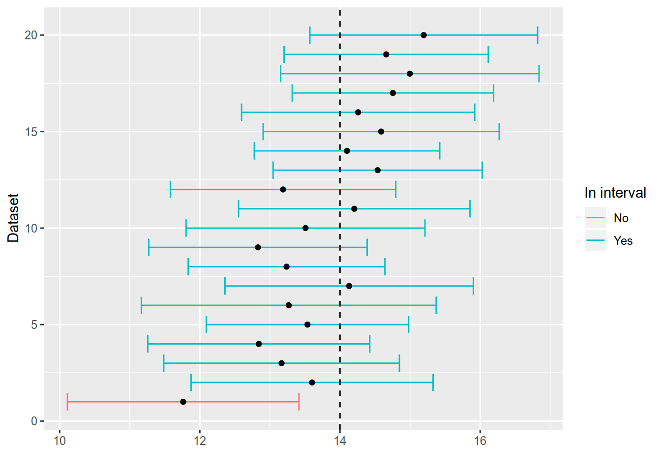
Out of 1000 datasets, the estimated confidence intervals contained the parameter \(\mu\) in 943 cases and failed to cover it in 57 cases. The percent of samples where the interval covered \(\mu\) is 94.3 quite close to the expected coverage rate of 95 percent.

Figure 7.1: Simulated confidence intervals. Only the first 20 intervals are shown. Intervals that do not contain $= 14 $ are coloured in red.
An important pattern in 7.1 that you should be aware of is that the confidence intervals are different in each sample just as the sample mean varied from sample to sample in (TODO XXX). This is because the endpoints of the interval are random variables, because they involve functions of the data (the sample mean and the standard deviation)!
Let us look at the confidence interval estimated for the hospital stay data: \([12.5, 15.7]\). When interpreting the confidence interval you man be tempted to say something like: the interval \([12.5, 15.7]\) contains the unknown parameter \(\mu\) with 95 percent probability. Please avoid doing this. In our setting \(\mu\) is a constant, some number that is unknown but not random. If you have doubts about that, look at the simulations. The sample mean changes from sample to sample but \(\mu\) is one and the same. It does not change with the data. So the statement that \(P(\mu \in [12.5, 15.7])\) does not make much sense. \(\mu\) is either in the interval or it is not in the interval. The probability statement is appropriate to the interval where the endpoints are random variables. It does not make any sense for the realised values of these random variables.
The confidence interval tries to cover the unknown parameter \(\mu\) (the expected value of a distribution) in 95 percent of all possible samples (95 percent probability). It is not an interval for the sample mean. As you can see in both 7.1 and (7.2) the sample mean is by construction always in the middle of the estimated confidence interval. Therefore the statement that the CI covers the sample mean with 95 percent probability is also nonsensical.