Chapter 4 Continuous distributions
In Chapter 3 we briefly discussed discrete random variables that could have a finite (or at most countably infinite) number of possible outcomes. It can be argued this type of random variables are sufficient to describe all real-world situations as we cannot measure anything with infinite precision. To illustrate it consider storing a real number in computer memory with infinite precision. This would require an infinite amount of memory which is infeasible. As an example of finite precision consider measuring the body temperature of flu patients. We can imagine that the temperature of a patient is a real number between 36 and 41 degrees Celsius but thermometers usually record it with a finite precision, e.g. \(36.1, 36.2,\ldots,39.9, 40\). However, it is often easier to work with random variables with a continuum of possible values. The present chapter reviews some basics of random variables with continuous distributions and introduces five special distributions: the uniform, normal, \(\chi^2\), t, and \(F\) distributions.
Now imagine a game where the possible outcomes are all real numbers in the interval [0, 1]. The number of possible values in that interval are uncountably many. In this course we will ignore the mathematical details that this entails. It is sufficient to say that we need to change the way we define probabilities for such games (random variables). The primary description of such games is the cumulative distribution function that assigns probabilities to events of the type \(X \leq x\).
Definition 4.1 (Cumulative distribution function, CDF) Let \(X\) be a random variable with possible values in the set of all real numbers \(\mathbf{R}\) (don’t confuse this with the software R). The function \(F(x)\)
All distributions that we will encounter in this course can also be described by a function \(f\) called the density function that we can integrate to obtain the distribution function \(F(x)\).
Let us illustrate the concepts of density and distribution functions using a simple yet important example. Imagine that you show up at a bus stop and wait for the bus to come. From experience you know that the waiting time will be between 0 and 1 minutes. Furthermore you know that the probability of waiting between 0 and 0.2, 0.2 and 0.3 minutes, is equal. A distribution that assigns a probability proportional to the length of an interval is the uniform distribution. Its density is constant over the whole support (set of possible values) of the distribution.
\[\begin{align} f(x) &= \begin{cases} 1 & \text{if } 0 \leq x \leq 1 \\ 0 & \text{otherwise.} \end{cases} \end{align}\]
![Density and CDF of the uniform distribution on [0, 1].](econometrics2020_files/figure-html/unnamed-chunk-14-1.png)
Figure 4.1: Density and CDF of the uniform distribution on [0, 1].
From the density function you can obtain the distribution function of the uniform distribution. First, on the interval \((-\infty, 0)\) the distribution function is zero, because the density is zero. \[\begin{align} F(x) = \int_{-\infty}^{0} f(t)dt = \int_{-\infty}^{0} 0dt = 0 \quad \text{for } x < 0. \end{align}\] On the interval [0, 1] the density is non-zero and we can integrate it to obtain.
\[\begin{align} P(X \leq x) = F(x) & = \int_{-\infty} ^ {x} f(t)dt \\ & = \int_{-\infty} ^ {0} f(t)dt + \int_{0} ^ {x} f(t)dt \\ & = 0 + \int_{0} ^ {a} 1 dx \\ & = [t]_{0}^{x} \\ & = x - 0 \\ & = x \tag{4.1}. \end{align}\]
On the interval \((1, +\infty)\) the density is again zero. \[\begin{align} F(x) & = \int_{-\infty} ^ {1} f(t)dt + \int_{1} ^ {x} f(t)dt \\ & = 1 + \int_{1} ^ {x} 0dt \\ & = 1 + 0 \\ & = 1. \end{align}\]
When we finally summarise all of the above the distribution function is: \[\begin{align} F(a) &= \begin{cases} 0 & \text{if } x < 0 \\ a & \text{if } 0 \leq x \leq 1 \\ 1 & \text{if } x > 1. \end{cases} \end{align}\]
Notice that the value of the integral in (4.1) is the area under the density function and in the case of the uniform distribution we can calculate it by simply using the formulas we know from basic geometry about the area of a rectangle. The area under the density function over the interval [0, 0.5] equals the product of the height of the rectangle (1) and the length of the interval (0.5):
\[\begin{align} F(0.5) = \underbrace{0.5}_{\text{length of interval}} \times \underbrace{1}_{\text{height of rectangle}} = 0.5. \end{align}\]
For a visualisation see 4.2.
\[\begin{align} F(x) = \begin{cases} 0 & \text{if } x < 0\\ 2x & \text{if } 0 \leq x \leq 0.5 \\ 1 & \text{if } x > 0.5. \end{cases} \tag{4.2} \end{align}\]
You can see the visualisation of both density and CDF functions of the [0, 0.5] uniform distribution in Figure 4.2.
![Density of the uniform distribution on [0, 0.5].](econometrics2020_files/figure-html/uniform-density-0-05-1.png)
Figure 4.2: Density of the uniform distribution on [0, 0.5].
\[\begin{align} P(1 \leq X \leq 1.5) & = P(X \leq 1.5) - P(X \leq 1) \\ & = 0.83 - 0.67 \\ & = 0.17. \tag{4.3} \end{align}\]
If you look closely at (4.3) you might be think that we have miscalculated the probability of \(1 \leq X \leq 1.5\). We have stated that \(P(1 \leq X \leq 1.5) = P(X \leq 1.5) - P(X \leq 1)\) instead of \(P(1 \leq X \leq 1.5) = P(X \leq 1.5) - P(X < 1)\). In the case of a discrete distribution you would be right. To see why both equations are correct here we will turn our attention to the difference between probability mass functions (discrete distributions) and density functions (continuous distributions).
Although the probability density function may resemble the probability mass function, both are quite different. The density function is not a probability function. There are two important differences. First, the density function can be greater than 1 as you can see in the example of a uniform random variable on the interval [0. 0.5] in 4.2. So the value of the density at any given possible value \(x\) cannot be the probability of occurrence of \(x\). Indeed, the probability of occurrence of any single value is zero, i.e. \(P(X = x) = 0\).
Formally we can show that \[\begin{align} P(X = x) & = \lim_{h \to 0^+}P(x - h < X \leq x) \\ & = \lim_{h \to 0^+}\left(F(x) - F(x - h)\right) \\ & = F(x) - \lim_{h \to 0^+}F(x - h) \\ & = F(x) - F(x) \\ & = 0 \tag{4.4}. \end{align}\]
Intuitively we can imagine the area under the density over a single point \(x\), which is zero. This might seem very surprising at first. After all, the result of a real-valued game must be some some real number. In the discrete case an event with probability zero is simply impossible. In the continuous case we only say that an event of zero probability does not occur almost surely. If you find it difficult to grasp this concept, think about a point in geometry. A line segment in geometry is a union of points and it has a non-zero length. Each individual point on that segment, however, has zero length.
An important consequence of (4.4) is that the probabilities of the two events \(X \leq x\) and \(X < x\) are equal. Remember that this only holds for continuous distributions with a zero probability for \(X = x\). \[\begin{align} P(X \leq x) = P(X < x). \end{align}\] The same holds for the events \(X \geq x\) and \(X > x\). \[\begin{align} P(X \geq x) = P(X > x). \end{align}\]
4.1 Expected value and variance
The two basic summaries of the distribution (expected value and variance) that we introduced for discrete random variables in Chapter 3 are also defined for continuous distributions.
The rules for working with the expected value and the variance presented in Chapter 3 are the same here (we will skip the proofs). The definitions of the expected value and the variance might seem completely different from the discrete case, but remember that the integral is actually the limit of a sum. It is important to remember that the expected value and the variance are fixed numbers, not random variables (for both continuous and discrete distributions).
\[\begin{align} E(X) & = \int_{-\infty}^{+\infty} xf(x) dx \\ & = \int_{-\infty}^{0} x \cdot 0 dx + \int_{0}^{1} x \cdot 1 dx + \int_{1}^{+\infty} 0 \cdot x dx \\ & = \left[\frac{x^2}{2}\right]_{0}^1 \\ & = \frac{1^2}{2} + \frac{0^2}{2} \\ & = \frac{1}{2}. \end{align}\]
To compute the variance it is easier if we use (3.9), so let us first compute the expected value of \(X^2\). \[\begin{align} E(X ^ 2) & = \int_{-\infty}^{+\infty} x^2 f(x) dx \\ & = \int_{-\infty}^{0} x^2 \cdot 0 dx + \int_{0}^{1} x^2 \cdot 1 dx + \int_{1}^{+\infty} x^2 \cdot 0 dx \\ & = 0 + \int_{0}^{1} x^2 \cdot 1 dx + 0 \\ & = \left[\frac{x^3}{3}\right]_{0}^{1} \\ & = \frac{1^3}{3} - \frac{0^3}{3} \\ & = \frac{1}{3} - 0\\ & = \frac{1}{3}. \end{align}\]
Finally we obtain the variance: \[\begin{align} Var(X) & = E(X ^ 2) - E(X) ^ 2 \\ & = \frac{1}{3} - \left(\frac{1}{2}\right)^2 \\ & = \frac{1}{3} - \frac{1}{4} \\ & = \frac{4 - 3}{12} \\ & = \frac{1}{12}. \end{align}\]
Notice (again) that the expected value and the variance are simply numbers. Not random variables.
Solution. \[\begin{align} E(X) & = 0.25 \\ Var(X) & = \frac{1}{24}. \end{align}\]
4.2 Quantile function
Until now we have learned how to compute the probabilities of events using the CDF F(x). Using it we can answer questions like: “What is the probability of \(X \leq 2\)?” by computing the CDF: \(F(2)\). Now let us invert the question and instead of asking about a probability given a number, let us ask about the number given the probability. For what real number \(q\) is the probability of the event \(X \leq q\) exactly \(0.2\)? Given the CFG we can invert it to answer the question.
Let us illustrate that with the simple CDF of uniform distribution on \([0, 0.5]\), see (4.2). \[\begin{align} F(x) = 2 x. \end{align}\] To find its inverse we can set it equal to some value \(p\) and solve for it. \[\begin{align} 2 x & = p \\ \implies x & = p / 2 \tag{4.5} \end{align}\]
The right hand side of (4.5) is what we call the quantile function of the distribution. \[\begin{align} Q(p) = p / 2. \end{align}\]
It enables us to answer questions like: “For which value \(a\) is the probability of the event \(X \leq a\) equal to 0.5?”. \[\begin{align} Q(0.5) = 0.5 / 2 = 0.25. \end{align}\]
You can substitute in the distribution function (4.2) with \(0.25\) to verify that the answer is correct.
We call Q(0.5) the 0.5 quantile of the distribution. Similarly Q(0.025) - the 0.025 quantile, Q(0.95) the 0.95 quantile, etc.
\[\begin{align} Q_{U[1, 3]}(0.05) & = 1.10 \\ Q_{U[1, 3]}(0.20) & = 1.40 \\ Q_{U[1, 3]}(0.90) & = 2.80 \end{align}\]
4.3 The normal distribution
The normal distribution is another continuous distribution and holds a prominent place in probability theory and statistics due to the central limit theorem (to be discussed later).
The density of the normal distribution is given by:
\[f(x) = \frac{1}{\sqrt{2 \pi \sigma ^ 2}} e ^ {-\frac{1}{2}(\frac{x - \mu}{\sigma}) ^ 2}, \quad x \in \mathbf{R}.\]
The formula might look somewhat intimidating but you will find that working with it is not that hard. For now it is sufficient to know that the density is non-negative for all real numbers and has two parameters: \(\mu\) and \(\sigma\). We will be using the normal distribution quite often and so it is convenient to introduce a special notation to refer to it. For a random variable following a normal distribution with parameters \(\mu\) and \(\sigma ^ 2\) we will simply write \(X \sim N(\mu, \sigma ^ 2)\).
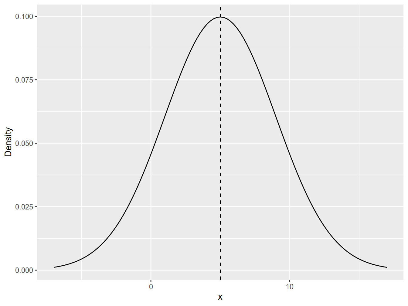
The normal distribution is symmetrical around \(\mu\):
Figure 4.3 shows a plot of the density of a \(N(5, 4)\). Note that the curve has a bell shape that is symmetrical around \(5\).

Figure 4.3: Density function of N(5, 4).
The symmetry of the density implies that the parameter \(\mu\) must be the expected value of the distribution. Here we will accept that without a formal proof. To motivate it but you can compare this statement with 4.2 where we derived the expected value of the uniform distribution (that is symmetrical, too).
\[\begin{align} E(X) = \int_{-\infty}^{+\infty} xf(x)dx = \mu. \tag{4.6} \end{align}\]
The second parameter of the distribution is \(\sigma ^ 2\) and it is easy to show that it equals the variance of the distribution. Again, we will accept this without a formal proof.
\[\begin{align} Var(X) & = \int_{-\infty}^{+\infty} \left(x - E(X)\right) ^ 2f(x)dx = \sigma ^2. \end{align}\]
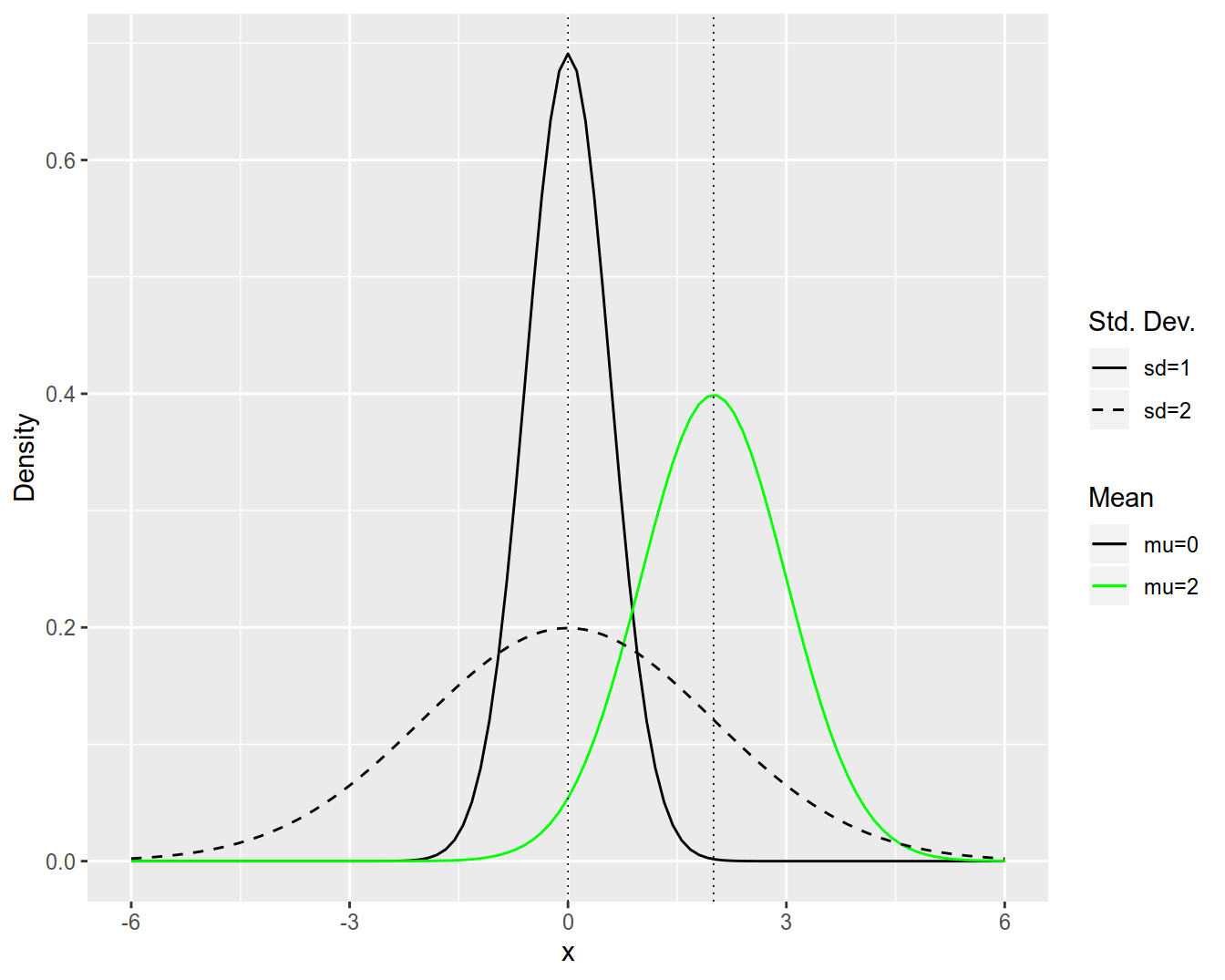
Both the expected value and the variance are summaries of the distribution function that measure specific aspects of that function. Think of the expected value as the centre of the distribution and of the variance as its spread. Experiment with the simulation here and see how the shape of the distribution changes with the values of \(\mu\) and \(\sigma ^ 2\). You will notice that changing \(\mu\) will shift the curve along the \(x\)-axis while changing \(\sigma\) affects its shape: the lower the standard deviation the steeper the bell curve. Figure 4.4 illustrates this for three normal distributions: \(N(0, 1), N(2, 1)\) and \(N(0, 4)\).

Figure 4.4: Plot of the \(N(0, 1), N(2, 1) and N(0, 4) densities.\)
4.3.1 Probabilities
Now that we are familiar with the shape of the normal distribution its time to learn how to compute probabilities and quantiles with R. The integral of the normal density cannot be computed analytically (as we did with the uniform distribution) and in earlier days you would have looked up the probabilities in long “probability tables”. Here we will use R for the computations. The function that we need is called pnorm and it computes the CFG at a given point x (first argument). The next two arguments are mean and sd. There you must supply the parameters \(\mu\) and \(\sigma\). Note that the pnorm function expects the standard deviation as an argument (\(\sigma\)) and not the variance (\(\sigma ^ 2\)). Furthermore, if you don’t specify mean and sd the function will assume the default values which are mean = 0 and sd = 1.
sd argument of pnorm.
## [1] 0.4012937\[\begin{align} P(X \leq 1.5) = 0.401 \end{align}\]
## [1] 0.5987063\[\begin{align} P(X > 1.5) = 1 - P(X \leq 1.5) = 1 - 0.401 = 0.599. \end{align}\]
pnLt2 <- pnorm(2, mean = 2 , sd = sqrt(4))
pnGtm1 <- pnorm(-1, mean = 2, sd = sqrt(4))

pnLt2 - pnGtm1
## [1] 0.4331928\[\begin{align} P(-1 < X < 2) & = P(X < 2) - P(X < -1) = \\ & = F(2) - F(-1) \\ & = 0.50 - 0.07 \\ & = 0.43. \end{align}\]
Before we conclude this section let us compute the probability of one and the same event under two different normal distributions: N(0, 1) and N(0, 4) (Figure 4.4). Imagine that you would like to purchase a house on the bank of a river and that you face a choice between two houses at two different rivers. The local hydrological information service advises you that on any given day the deviations from the normal level of the rivers (in meters) are described by \(N(0, 1)\) for the first river and \(N(0, 2)\) for the second one. Both houses are situated about 2 meters above the normal river level and you are particularly interested in the probability of the event \(X > 2\) (your house gets flooded). What are the probabilities of these events?
\[\begin{align} P_{N(0, 1)}(X > 2) & = 0.02 \quad \text{first river}\\ P_{N(0, 2)}(X > 2) & = 0.16 \quad \text{second river}. \end{align}\]
The probability of a flood is noticeably higher under the distribution with the higher variance. Your final choice of a house would of course depend on its price and multiple other factors, but at the second river you should expect to be cleaning up flood damage on about 16 out of 100 days (assuming independence).
4.3.2 Quantiles
Calculating quantiles for normal distributions is easy with the R function qnorm. It expects a probability as its first argument and returns a real number. As with pnorm you need to specify the mean and sd arguments.
## [1] -1.84897\[\begin{align} P(X \leq -1.85) = 0.05. \end{align}\]
Find the number \(a\) for that the probability of \(X > a\) equals 0.1.
## [1] 3.219712\[\begin{align} P(X > a) & = 1 - P(X \leq a) = 1 - 0.1 = 0.9 \\ P(X \leq 3.220) & = 0.9 \\ \implies a & = 3.220. \end{align}\]
4.4 Chi square distribution
The \(\chi^2\) distribution commonly arises in statistical tests. Unlike the normal distribution, the \(\chi^2\) distribution has a single parameter called the degrees of freedom.
\[\begin{align} Z_1 ^2 + Z_2 ^ 2 + \ldots + Z_n^2 \sim \chi^2(n) \tag{4.7}. \end{align}\]
It can be shown that the expected value of a \(\chi^2(n)\) distributed variable is equal to the degrees of freedom of the distribution.
\[\begin{align} E(X) = n. \end{align}\]
It can be shown that if the variables in the sum (4.7) are subject to \(k\) linearly independent restrictions of the form:
\[\begin{align*} a_{11} Z_1 + a_{12} Z_2 + \ldots + a_{1n} Z_n & = b_1 \\ & \vdots \\ a_{kn} Z_1 + a_{22} Z_2 + \ldots + a_{kn} Z_n & = b_k \end{align*}\]
then the sum of the \(n\) squared variables follows a \(\chi^2\) distribution with \(n - m\) degrees of freedom.
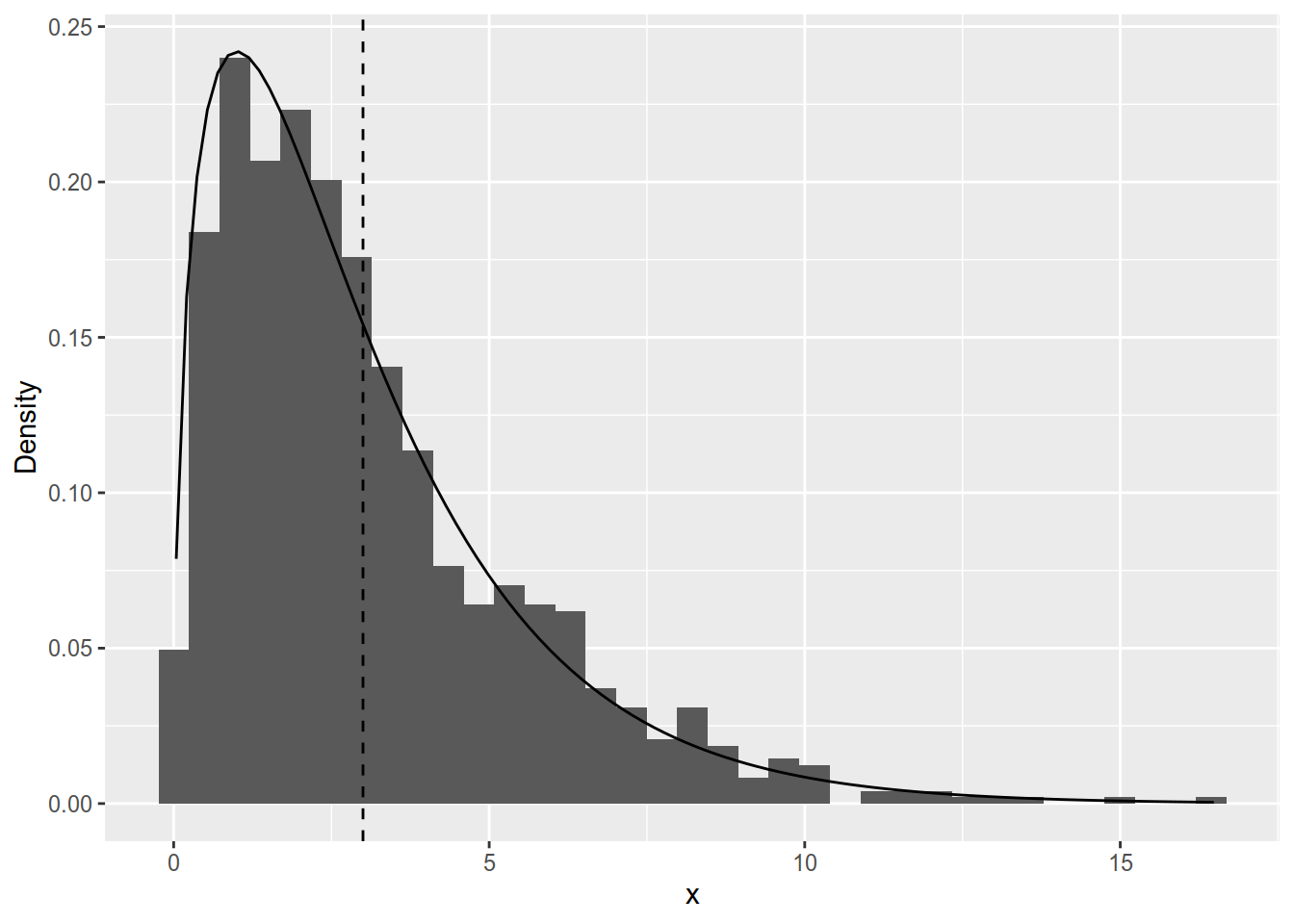
Figure 4.5 shows a simulation of 1000 realisations from the \(\chi^2(2)\). Notice that the values are all non-negative due to the squares in (4.7) and that the distribution is not symmetrical but is skewed to the right.

Figure 4.5: Histogram of 1000 realisations from a \(\chi^2(3)\) distribution. The vertical line is drawn at 3 (the expected value of the distribution).
You can experiment with this simulation to see how the shape of the \(\chi^2\) distribution changes with the degrees of freedom here.
4.5 t-distribution
The t-distribution is another distribution very common in statistical tests. Its density function is quite involved and we will not present it here. Instead we will visualise its density and compare it to the standard normal distribution.
The \(t\)-distribution with \(n\) degrees of freedom arises as the ratio between a standard normal random variable Z and a the square root of a \(\chi^2\) distributed variables.
Definition 4.6 (t distribution) Let \(Z \sim N(0, 1)\) and \(X \sim \chi ^ 2 (n)\) be two independent random variables. The ratio between \(Z\) and the square root of \(X / n\) follows a t-distribution with \(n\) degrees of freedom.
\[\begin{align} T = \frac{Z}{\sqrt{X / n}} \sim t(n). \end{align}\]
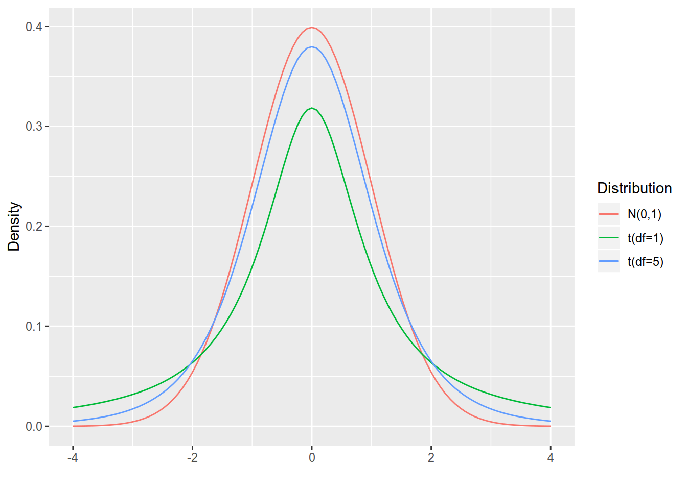
Figure 4.6: Densities of the standard normal and t-distributions with 1 and 5 degrees of freedom.
For this course it is sufficient to know that the t distribution has an expected value of zero for all degrees of freedom. It is symmetric around 0 and has greater probability for extreme events than the standard normal distribution (Figure 4.6). The difference from the standard normal is largest for small degrees of freedom and gets smaller for high degrees of freedom.
4.5.1 Probabilities
To compute probabilities of the t distribution we will use the pt function which accepts a real number \(x\) as its first argument and returns the probability for the event \(X \leq x\). Note that you must specify the degrees of freedom under its df argument, otherwise
R will throw an error complaining about missing arguments.
## [1] 0.2612501\[\begin{align} P_{t(4)}(T < -0.7) = 0.26. \end{align}\]
## [1] 0.321665\[\begin{align} P_{t(4)}(T > 0.5) = 1 - P(T < 0.5) = 1 - 0.68 = 0.32. \end{align}\]
4.5.2 Quantiles
We will use the qt function to compute quantiles of the t-distribution. It accepts a probability as its first argument and returns a real number. As with pt you are required to specify the df argument. We will be using quantiles of t-distributions quite often, therefore we will introduce a shorthand notation. For the \(\alpha\) quantile of a t-distribution with \(n\) degrees of freedom we will write \(t_{\alpha}(n)\). For example for the 0.05 quantile of the t-distribution with 30 degrees of freedom we will write \(t_{0.05}(30)\).
## [1] -0.7406971\[\begin{align} P_{t(4)}(T \leq t_{0.25}(4)) = 0.25. \\ t_{0.25} = -0.741 \end{align}\]
\[\begin{align} P_{t(4)}(T > a) = 0.3 \end{align}\]
Finding \(a\) such that \(P_{t(4)}(T > a) = 0.3\) is equivalent to finding \(P_{t(4)}(T \leq a) = 0.7\). The latter is by definition the 0.7 quantile of the t-distribution with 4 degrees of freedom. Let us compute it using R.
## [1] 0.5686491\[\begin{align} & P_{t(4)}(T < t_{0.7}(4)) & = 0.7 \\ \implies & P_{t(4)}(T > t_{0.7}(4)) & = 0.3 \\ \implies & P_{t(4)}(T > 0.57) & = 0.3 \\ \implies & a = t_{0.7}(4) & = 0.57. \end{align}\]
4.5.3 Comparison with the standard normal distribution
Now that we know how to compute probabilities using both the t-distribution and the normal distribution we can compare the distributions. Consider again the case of two rivers from Section 4.3.1. Let deviations from the normal level of the first river follow a standard normal distribution as before. This time we will assume that the deviations of the second river follow a t-distribution with one degree of freedom. Which river has a higher probability of flooding your house?
## [1] 0.02275013## [1] 0.1475836\[\begin{align} P_{N(0,1)}(X > 2) = 0.0228 \\ P_{t(1)}(X > 2) = 0.1476. \end{align}\]
Notice that under the \(t(1)\) distribution the probability for \(X > 2\) (flood) is much greater than under the standard normal distribution. This difference is smaller for t-distributions with higher degrees of freedom.
## [1] 0.02410609\[\begin{align} P_{t(100)}(X > 2) = 0.0241. \end{align}\]
4.6 F-distribution
Another distribution that is very common in statistical tests is the F distribution. It arises as the ratio of two independent \(\chi^2\) variables scaled with their respective degrees of freedom.
We say that the ratio \(F\) follows a F distribution with \(n\) nominator degrees of freedom and \(m\) denominator degrees of freedom.