Chapter 5 Point Estimation

Imagine again the lottery game from the beginning of Chapter 2. The whole theory that we have developed so far requires knowledge of the rules of the game (i.e. its probability function) in order to compute its expected value, variance, etc. What happens though if we have no idea about how the lottery (or any other process) actually works?

One way to learn the rules of the game is to observe it. In the case of the lottery to observe it means to play it and learn from the results. In the case of the corona virus patients this means to measure the incubation periods of selected patients learn about the the nature of the virus.

In the case of the lottery consider buying \(n\) tickets and denote the (yet unknown) value of each ticket with \(X = (X_1, X_2, \ldots, X_n)\). We call the vector of random variables \(X\) a sample from the game (or patients in the other example). For the purposes of all discussions we will assume that the variables are identically distributed. This means that we assume that all \(X_i\) have one and the same distribution (i.e. we play one and the same game). Second, we assume that the variables are independent. Put informally this means that the result from the first game \(X_1\) (whether it wins 0, 1, or 2 EUR) does not change the rules of the game. In other words, the distribution of the winnings of the next ticket \(X_2\) must not depend on the outcome of \(X_1\).

Sometimes it can be hard or unnecessary to learn all rules of the game by observing it (in the lottery example this would amount to learn the probabilities of each outcome). Quite often it will be sufficient if we learn some special aspects of the rules (the distribution). In the previous chapters we introduced two important summaries of distribution functions (rules of the game): the expected value and the variance. In the next two chapters we will show how to estimate these using a sample.

In the following we will assume that the sample comes from a normal \(N(\mu, \sigma^2)\) distribution. Notice that in this case learning the expected value and the variance amounts to learning everything as the normal distribution is completely determined by \(\mu\) and \(\sigma ^ 2\).

Let us assume that the \(n = 114\) patients in our dataset are a random sample from one and the same normal distribution \(N(\mu, \sigma ^ 2)\). Let us write \(X_1\) for the (yet unknown) value of the incubation period of the first selected patient, \(X_2\) for the incubation period of the second selected patient and \(X_n\) the incubation period of the last patient. We can write this more compactly as a vector of random variables: \(X = (X_1, X_2,\ldots,X_n)\) with \(n\) being the total number of selected patients. When we actually measure the incubation periods of all patients in our sample we see a realisation of the random variables: \(x_1, x_2,\ldots,x_n\). These are the values that you see in the R data frame (table) linton.

We will use uppercase letters to denote random variables (games) and lowercase letters for concrete values (realisations). Once the incubation periods are measured, the observed values are not random. They are simply numbers that we can use in R for computations. In contrast, you cannon compute the mean of random variables with R the way you do this with concrete values. The difference is important for the study of the properties of functions of the data (statistics). When we study these properties we need to think about all possible samples that we could obtain, not only about the (usually) one sample that we happen to observe.

Take for example the incubation time of the first patient. It is 2 days and there is nothing random in this number. Therefore it makes little sense to ask about its expected value (it is 2) or its variance (it is zero). It is the sampling mechanism that is random, not the concrete realisations. In the lottery example you can think of the random variables as holding a lottery ticket in your hand. Before you scratch the surface you don’t know how much you win, at best you have an idea about the distribution of the possible winnings. After you scratch the ticket you see the actual (realised) value of your ticket (lowercase letter) is an amount in EUR (not random).

5.1 Sample mean

In this chapter we will discuss the properties of the sample mean as an estimator of the expected value of a normal distribution. Here we will examine its properties but we will not discuss general methods like the method of moments or maximum likelihood. In Section 8.1 we show that the sample mean is the OLS estimator for the expected value. For a normal sample it can be shown that it is the maximum likelihood estimator for the expected value as well.

We will be using the sample mean to estimate \(\mu\). To emphasise that we will put a hat over \(\mu\) to be able to tell apart the parameter (\(\mu\)) and the estimator (\(\hat{\mu}\)) for that parameter.

\[\begin{align} \hat{\mu} = \bar{X} = \frac{1}{n}\sum_{i = 1} ^ {n} X_i. \tag{5.1} \end{align}\]

It is important to see that that \(\hat{\mu}\) (the estimator) is a function of the data \((X_1, \ldots, X_n)\) and it will therefore change when the data changes (i.e. when we observe another sample). The parameter \(\mu\) does not change with the data.

When we have a concrete sample (\(x_1,\ldots,x_n\)) we can compute the realised value of \(\hat{\mu}\).

\[\begin{align} \hat{\mu} = \bar{x} = \frac{1}{n}\sum_{i = 1} ^ {n} x_i. \tag{5.2} \end{align}\]

Notice that unlike the case of the sample variables \(X_i\) and \(x_i\) (uppercase and lowercase letters) we use the same symbol (\(\hat{\mu}\)) for both the function of the data (the estimator) and its realised value (the estimate). You should be able to infer from the context whether we are talking about the estimator or the estimate. Think about the function in (5.1) as the average value of a bunch of \(n\) lottery tickets before you know how much each of these tickets is worth. Think of equation (5.2) as your actual average winnings per ticket (when you already know how much each ticket has won).

Now that we have determined that we will estimate the expected value using the sample mean we should be able to say something about its properties. When we see a sample (e.g. the patients or the lottery tickets) we know that it is not the only sample that we could have obtained. Repeating the experiment (selecting patients, buying tickets) will result in a different sample. When we are thinking about how to construct an estimator we need to think about all possible samples. In other words we face a question about the sampling distribution of the sample mean.

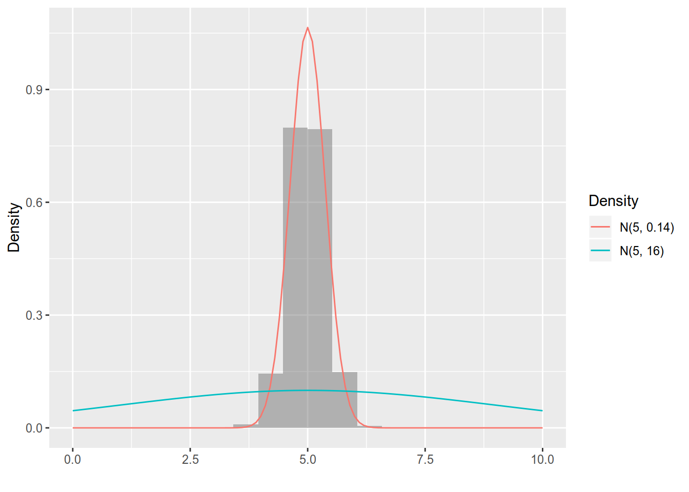
## `summarise()` ungrouping output (override with `.groups` argument)

To gain a better understanding about how the sample mean varies over a large set of possible samples we will run a simulation. We generate \(B = 1000\) samples of size \(n=114\) from the \(N(5, 4^ 2)\) distribution. For each sample we compute the mean and the result are \(1000\) means (one per sample) that are visualised in a histogram in 5.1 and summarised in Table 5.1.

Table 5.1: Summary of the sample means for 1000 datasets with sample size n= 114 from \(N( 5 , 4 ^2).\)

Min	Q25	Mean	Median	Q75	Max
3.718463	4.73426	4.999517	4.998185	5.256482	6.145799

Figure 5.1: Summary of the sample means for 1000 datasets with sample size \(n=114\). Overlayed are the densities of the sample mean \(N(5, 0.14)\) (red) and the original distribution \(N(5, 4^2) (blue).\)

There are three important things to learn from this simulation. First, we see that the sample mean is different in every sample. Although they are different, there appears to be some pattern in their distribution (more on that later). Second, we see that the average of the 1000 means (5) (yes, this is the mean of means…) is quite close to the known expected value of \(5\). Half of the means are quite close to the expected value . Third, there are samples where the sample mean was far away from the expected value: look at the minimum and the maximum in Table 5.1.

When we observe a sample we have no idea which one of all possible samples we have selected. We can be very unlucky to have selected a sample that produces a mean that is very far away from the expected value. In other words our conclusion about \(\mu\) is uncertain.

While there may be no real defence against bad luck, we can at least describe the uncertainty of our estimator by studying its sampling distribution. We have done the first step in the simulation in Figure 5.1. Next we will derive its distribution analytically. Before we do that we will introduce a general criterion that can help us measure the “goodness” of an estimator. So what is a “good” estimator?

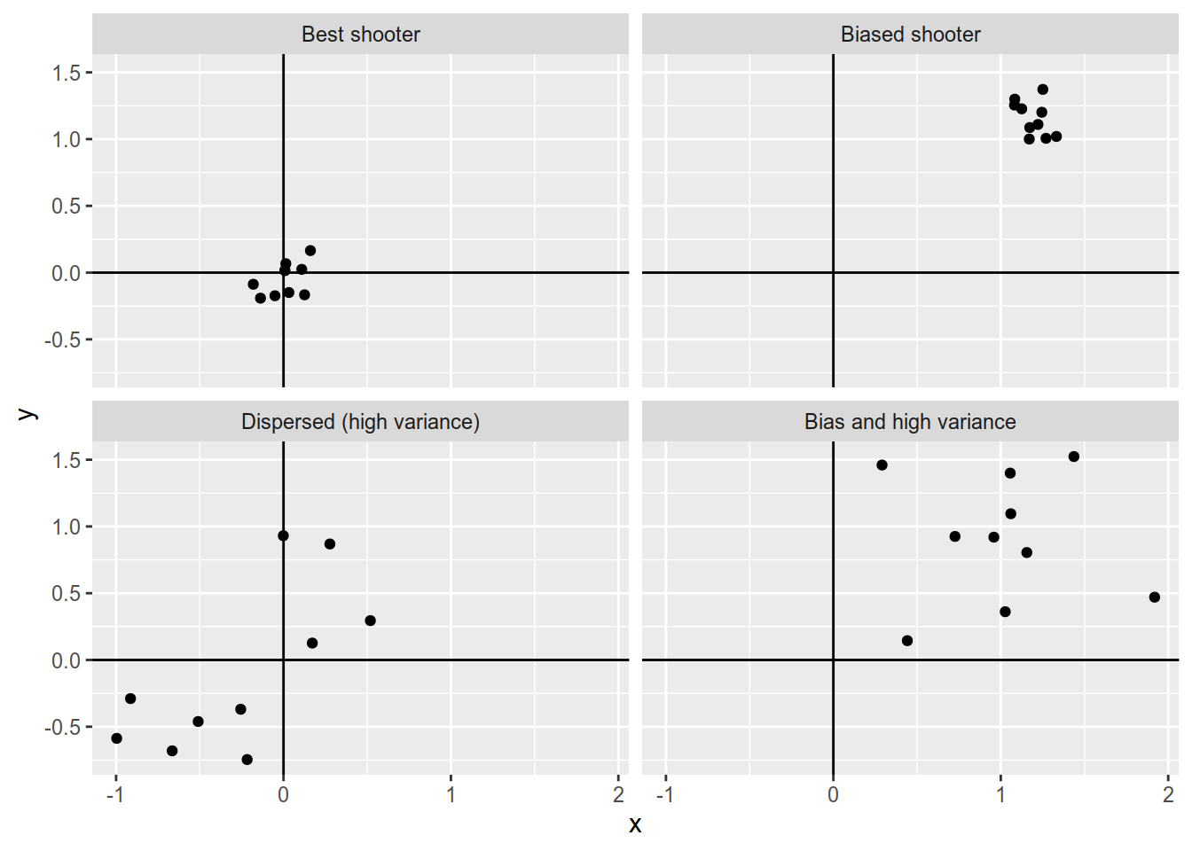
Think again about what we are doing. Based on an observed sample we try to “guess” the value of the (unknown) \(\mu\). We can do this in a lot of different ways but in statistics we usually use some function of the data. We are in a situation very much alike to a shooter trying to hit a target. Intuitively, a good shooter will hit the target at least on average, meaning that her shots will land around the bull’s eye. Sometimes she may hit slightly above the centre, sometimes slightly below it, but on average her shots should not systematically land far from it. However, there are different ways to hit the target “on average”. A shooter who has large deviations above and below the target will have the same average than a shooter whose shots land close to each other (small deviations above and below). The average does not tell you how different the shots are. This is a task for the variance.

Look at Figure 5.2 where we compare four different shooters. The first (top left) one is quite experienced and hits the target (the parameter) with little difference (low variance) between the shots (samples). The next one (bottom left) appears to be an inexperienced shooter who shoots wildly over and below the target (high variance). On average the these deviations of her shots below and above the target cancel out but we would not say that she is a good shooter. The third shooter (top right) also appears to be experienced as the shots are concentrated (low variance) but it seems that she is systematically doing something wrong, because all shots land far away from the target. The last shooter is both inexperienced and does not hit the target on average.

Figure 5.2: Simulation of 10 shots by four shooters aiming at the target at (0, 0).

A criterion that combines both bias (not hitting the target on average) and variance (large differences between shots) is the mean squared error of the estimator.

Definition 5.1 (Mean squared error) The mean squared error is defined as the expected squared difference of the estimator and the parameter. In the case of the expected values this is

\[\begin{align} MSE(\hat{\mu}) = E(\hat{\mu} - \mu) ^ 2 = \underbrace{Var(\hat{\mu})}_{\text{variance}} + (\underbrace{E(\hat{\mu} - \mu)}_{\text{bias}}) ^ 2. \end{align}\]

Applied to the shooters from Figure 5.2 the best shooter has the lowest MSE, because she has low bias (average deviation from the target) and low variance (difference between the shots).

Let us now return to the sample mean and derive its expected value (and hence its bias) and its variance. Using (3.6) and (3.4) we can show that the expected value of the sample mean is:

\[\begin{align} E(\hat{\mu}) & = E(\frac{1}{n}\sum_{i = 1} ^ {n} X_i) \\ & = \frac{1}{n} \sum_{i = 1} ^ {n} E(X_i) \\ & = \frac{1}{n} \sum_{i = 1} ^ {n} \mu \\ & = \frac{1}{n} n \mu \\ \implies E(\hat{\mu}) & = \mu \tag{5.3} \end{align}\]

We say that it is an unbiased estimator for \(\mu\), because its bias is zero:

\[\begin{align} E(\hat{\mu} - \mu) & = E(\hat{\mu}) - \mu \\ & = \mu - \mu \\ & = 0. \end{align}\]

This means that the distribution of the sample mean is centred at \(\mu\) (the value we are trying to hit). It is important to understand that does not imply that our estimator will be equal to \(\mu\) (look again at the simulation summary in Table 5.1).

Using (3.8) and (3.7) we can derive the variance of the sample mean: \[\begin{align} Var(\bar{X}) & = Var\left(\frac{1}{n}\sum_{i = 1} ^ n X_i\right) \\ & = \left(\frac{1}{n}\right) ^ 2 Var\left(\sum_{i = 1} ^ n X_i\right) \\ & = \frac{1}{n^2}\sum_{i=1}^n Var\left(X_i\right) \\ & = \frac{1}{n^2}\sum_{i=1}^n \sigma^2 \\ & = \frac{n\sigma^2}{n^2} \\ & = \frac{\sigma ^2}{n} \tag{5.4} \end{align}\]

It can be shown (Casella and Berger 2001, 215) that the sum of independent normally distributed random variables also follows a normal distribution, so finally we obtain that \(\bar{X} ~ N(\mu, \sigma ^ 2 / n)\). Notice that the variance of the sample mean decreases with increasing sample size \(n\). Intuitively you can think about \(n\) as the amount of information that we use in the estimator. More information about the unknown distribution \(N(\mu, \sigma ^ 2)\) enables us to estimate \(\mu\) with lower uncertainty. In the shooters example you can think about how grounded a shooter is before she fires. A small sample size will resemble someone shooting from the hip (not well grounded). A large sample size will resemble someone shooting from a stable position.

5.2 Sample variance

Up to now we have learned about the sampling distribution of the sample mean. The normal distribution has one more parameter that we need to estimate, though. For the sake of brevity we will only present an estimator and state its sampling distribution without explicitly deriving it.

Definition 5.2 (Sample variance) Let \(X = (X_1,\ldots,X_n)\) be a random sample. The (corrected) average squared deviation of \(X_1,\ldots,X_n\) from their sample mean \(\bar{X}\) is called the sample variance:

\[\begin{align} S^2(X) = \frac{1}{n - 1}\sum_{i = 1} ^ {n} (X_i -\bar{X}) ^ 2. \tag{5.5} \end{align}\]

By definition the sample variance is always non-negative. It is zero only if and only if all values are equal (i.e. all values are equal to their mean).

Definition 5.3 (Sample standard deviation) The square root of the sample variance \(S(X) = \sqrt{S^2(X)}\) is called the standard deviation of \(X\).

While the sample mean is a measure of the centre of a set of data points, the sample variance measures how different the data points are (compared to each other).

Example 5.1 Compute the sample variance and the sample standard deviation of \(x = (x_1 = 0, x_2 = 1, x_3 = 2)\).

Solution. First compute the average of \(x\). \[\begin{align} \bar{x} = \frac{1}{3}(0 + 1 + 2) = \frac{3}{3} = 1. \end{align}\] then apply 5.2: \[\begin{align} S^2(x) & = \frac{1}{n - 1} \left( (\underbrace{x_1 - \bar{x}}_{\substack{\text{deviation of} \\ x_1 \text{ from } \bar{x}}}) ^ 2 + (\underbrace{x_2 - \bar{x}}_{\substack{\text{deviation of} \\ x_2 \text{ from } \bar{x}}}) ^ 2 + (\underbrace{x_3 - \bar{x}}_{\substack{\text{deviation of} \\ x_3 \text{ from } \bar{x}}}) ^ 2 \right) \\ & = \frac{1}{3 - 1}\left(0 - 1) ^ 2 + (1 - 1) ^ 2 + (2 - 1) ^ 2\right) \\ & = \frac{1 + 0 + 1}{2} \\ & = 1 \\ S(x) & = \sqrt{S^2(x)} = \sqrt{1} = 1. \end{align}\]

Example 5.2 Compute the sample variance of \(y = (y_1 = -1, y_2 = 2, y_3 = 5)\).

Solution. \[\begin{align} S^2(y) = 9 \\ S(y) = 3. \end{align}\]

Example 5.3 Compute the sample variance and sample standard deviation of z = (z_1 = 1, z_2 = 1, z_3 = 1).

Solution. \(S^2(z) = 0, S(z) = 0\).

Compare the numbers in the three sets from the last examples. You should notice that the variance is higher in the second example relative to the other two. This reflects the fact that the numbers in that set are more spread out compared with the other two (the numbers are more heterogeneous in other words). The variance in the last example is exactly zero, because there is no difference between the elements of the set (all numbers are equal).

5.2.1 Distribution of the sample variance

We already know that the sample mean is a random variable, because it depends on the data. The same holds for the sample variance. The following theorem establishes the sampling distribution of the sample variance.

Theorem 5.1 Given a sample of independen normal variables \(X_1,\ldots,X_n\), \(X_i \sim N(\mu, \sigma ^2)\):

\[\begin{align} \frac{n - 1}{\sigma ^ 2} S^2(X) \sim \chi^2(n - 1) \end{align}\] where \(S^2(X)\) is the sample variance of \(X\):

\[\begin{align} S^2 = \frac{1}{n - 1} \sum_{i = 1}^n (X_i - \bar{X}) ^ 2. \tag{5.5} \end{align}\]

Note that the degrees of freedom in 5.1 are \(n - 1\) and not \(n\). The proof of the theorem is beyond the scope of this course but note that the summands in (5.5) are not independent. These are deviations from the sample mean and therefore sum to zero.

\[\begin{align} \sum_{i = 1} ^ n (X_i - \bar{X}) & = \sum_{i = 1} ^ n X_i - \sum_{i = 1} ^ n \bar{X}\\ & = \frac{n}{n}\sum_{i = 1} ^ n X_i - n \bar{X}\\ & = n\bar{X} - n \bar{X} \\ & = 0. \end{align}\]

Using Theorem 5.1 we can see that the sample variance is an unbiased estimator for \(\sigma ^ 2\). To show that we use the property of the \(\chi^2\) distribution that its expected value equals the degrees of freedom.

\[\begin{align} E\left(\frac{n - 1}{\sigma ^ 2} S^2(X) \right) = n - 1 \\ \implies E(S^2(X)) = \sigma ^ 2. \end{align}\]

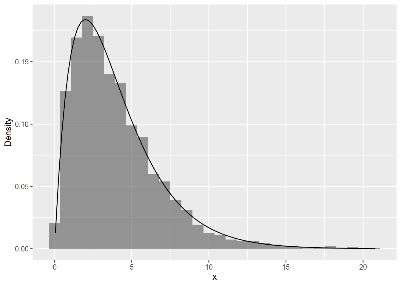
Figure 5.3 shows a simulation using 5000 samples from the \(N(0, 4)\) distribution. Notice that the variance of the distribution (\(\sigma ^ 2 = 4\)) does not change from sample to sample. The sample variance does change, though, because it is a function of the data.

Figure 5.3: Distribution of \(\frac{n - 1}{\sigma ^ 2}S^2(X)\) for 5000 samples from N(0, 4) of size n = 5. Overlayed is the density of the \(\chi^2(5 - 1).\)

References

Casella, George, and Roger Berger. 2001. Statistical Inference. Cengage Learning, Inc. https://www.ebook.de/de/product/3248529/george_university_of_florida_casella_roger_arizona_state_university_berger_statistical_inference.html.