Chapter 6 Hypothesis testing
Consider again the covid-19 incubation times data. A leading expert claims that the expected incubation period is much higher than our estimate of 5.39 days and is actually 8 days. Can we check whether her claim is consistent with the our observed data? For that purpose we will conduct a statistical test.
Statistical tests work just as a court deliberating whether to convict a person accused of a crime. The court generally does not know whether the accused is actually guilty. All it can do is to examine the evidence pointing to the person’s guilt and weight it against some standard of certainty (e.g. beyond all reasonable doubt, preponderance of evidence, balance of probabilities etc.).
The court bases its decision on the evidence presented by both sides of the process: the prosecution and the defence. The defence claims innocence of the crime (null hypothesis), the prosecution summarises the evidence against the claim of the defence and presents it to a jury (or a judge/panel of judges) who weight the evidence against a standard of proof and make a decision. The jury can either reject the claim of the defence and convict or fail to reject it given the evidence (not convict). Note that a failure to convict rarely amounts to a finding of innocence. This simply means that the evidence was not convincing enough. Regardless of how good the court is, assuming uncertainty about the person’s guilt, it is always possible to make a wrong decision. A court can make two kinds of errors: to convict an innocent person or to release a guilty one. Releasing an innocent person and convicting a guilty one are obviously not errors.
The evidence in our case is the data on the length of incubation periods, so it is already collected. Let us denote the incubation periods of the \(i=1,\ldots,n = 114\) patients with (\(X_1,\ldots,X_n\)).
We want to test the statement that the expected incubation period is \(8.00\) days. Let us call this statement the null hypothesis \(H_0\) for short.
6.1 t-statistic
Next we need a statistic (a function of the data) that can summarise the evidence and present it to the jury. We will skip the whole derivation here (it is not trivial) and will use the following test statistic
\[\begin{align} T(X_1,\ldots,X_n, \mu_0) = \frac{\bar{X} - \mu_0}{S(X) / \sqrt{n}} \tag{6.1} \end{align}\]
where \(S(X)\) is the sample standard deviation of \(X\) (see (5.5)) and \(n\) is the sample size.
Because it is a function of the data, the function \(T\) is a random variable that has a sampling distribution. We are particularly interested in the sampling distribution of \(T\) assuming that the sample comes from a \(N(\mu_0, \sigma ^ 2)\) distribution. Note that the latter implies that the null hypothesis is true. We will refer to this distribution as the distribution of \(T\) under the null hypothesis in order to avoid repeating every time: “assuming that H_0 is true the distribution of T is …”. Under \(H_0\) the statistic follows a t-distribution with \(n - 1\) degrees of freedom. To see that rewrite the statistic in the following way:
\[\begin{align} T(X_1,\ldots,X_n, \mu_0) & = \frac{\bar{X} - \mu_0}{S(X) / \sqrt{n}} \\ & = \sqrt{n} \frac{\bar{X} - \mu_0}{S(x)} \\ & = \sqrt{n} \frac{\frac{\bar{X} - \mu_0}{\sigma}}{\frac{S(X)}{\sigma}} \\ & = \frac{\frac{\bar{X} - \mu_0}{\sigma / \sqrt{n}}}{\frac{S(X)}{\sigma}} \\ & = \frac{\frac{\bar{X} - \mu_0}{\sigma / \sqrt{n}}}{\sqrt{\frac{(n - 1)S^2(X)}{(n - 1)\sigma ^ 2}}} \tag{6.2} \end{align}\]
From (6.2) we need to see three things. First, under \(H_0\) the nominator follows a standard normal distribution. We know that from (5.3) and (5.4) but let us show this here again. The expected value of the nominator is zero:
\[\begin{align} E\left(\frac{\bar{X}- \mu_0}{\sigma /\sqrt{n}}\right) & = \frac{1}{\sigma / \sqrt{n}}\left(E(\bar{X}) - \mu_0\right) \\ & = \frac{1}{\sigma / \sqrt{n}} \left(\mu_0 - \mu_0\right) \\ & = 0. \tag{6.3} \end{align}\]
and its variance is 1:
\[\begin{align} Var\left(\frac{\bar{X}- \mu_0}{\sigma /\sqrt{n}}\right) & = \frac{Var(\bar{X})}{\sigma ^ n} \\ & = \frac{\sigma ^ 2 / n}{\sigma ^ 2 / n} \\ & = 1. \tag{6.4} \end{align}\]
Second, if the sample does not originate from a normal distribution with mean \(\mu_0\) (i.e. if \(H_0\) is not true) the nominator does not follow a standard normal distribution, because its expected value is not zero.
Third, the term in the denominator under the square root is a \(\chi^2\) distributed variable divided by \(n - 1\), its degrees of freedom (see Theorem 5.1). Both facts fit into the definition of a t-distribution in definition 4.6. That definition also requires that the nominator and denominator are independent and this is indeed the case here, but the proof is beyond our scope.
Let us summarise this result in a theorem.
\[\begin{align} T(X_1,\ldots,X_n, \mu_0) = \frac{\bar{X} - \mu_0}{S(X) / \sqrt{n}} \sim t(n - 1). \tag{6.5} \end{align}\]
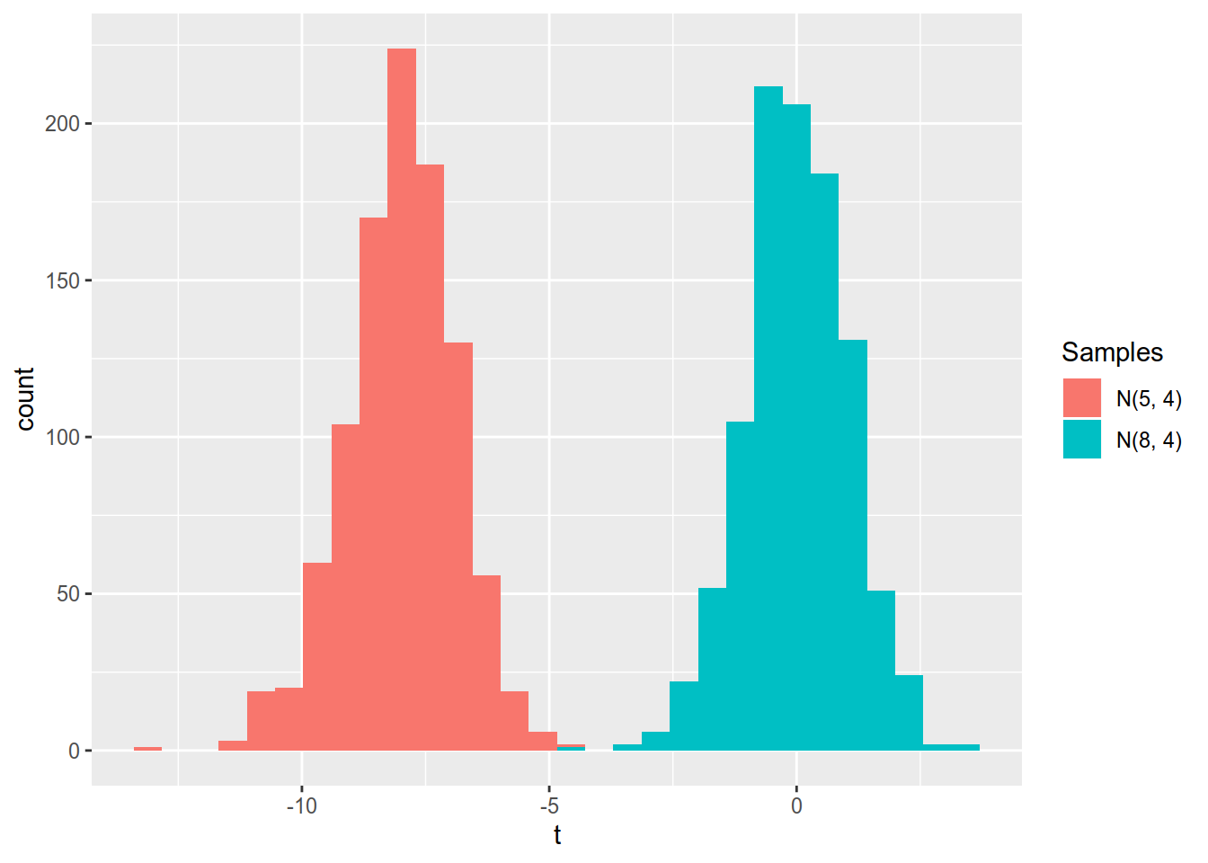
## `summarise()` ungrouping output (override with `.groups` argument)Intuitively, if the sample comes from \(N(\mu_0, \sigma ^ 2)\) then we expect to see small values of the t-statistic that are near 0 (its expected value). “Large” values of the t-statistic indicate that the sample may not have originated from \(N(\mu_0, \sigma ^ 2)\). To see that, look at the simulation of t-statistics computed at \(\mu_0 = 8\) for 2000 samples generated from two different normal distributions: \(N(8,4)\) and \(N(5,4)\) (1000 samples per distribution) in Figure 6.1.

Figure 6.1: Distributions t-statistics calculated at mu_0 = 8 for N(8,4) and N(5,4) . Based on 1000 samples from each distribution.
The t-statistics are concentrated around zero for the \(N(8,4)\) distribution but are far away from it for the samples generated from \(N(5,4)\).
6.2 Two sided tests
Until now we have shown how to compute the t-statistic, our summary of the evidence (the data) and we have argued that values of that statistic that are far away from zero are inconsistent with \(H_0\). In order to make a decision to reject or not to reject the null hypothesis we need to weight the strength of the evidence against \(H_0\), the t-statistic, against a standard of proof.
Look again at the statement that we would like to test with our data: “The expected incubation period is 8 days”. An alternative to this statement can be “The expected incubation period is not equal to 8 days”. Written in shorthand notation the null hypothesis (\(H_0\)) and this alternative (\(H_1\)) look like:
\[\begin{align} H_0 & = \mu_0 \tag{6.6}\\ H_1 & \neq \mu_0. \end{align}\]
In our example the average incubation period is 5.395 days, the standard deviation is 4.534 days and the sample size is \(n = 114\). With this three pieces we can compute the value of the t-statistic at \(\mu_0 = 8\):
\[\begin{align} t = \frac{5.39 - 8}{4.53 / \sqrt{114}} = -6.135. \end{align}\]
Now we must decide whether \(t = -6.135\) is a large enough deviation from zero in order to reject \(H_0\). Let us construct a region of values called the rejection region. If the value of the t-statistic falls in that region we reject \(H_0\). From (6.6) we see that both large negative small and large positive values of the statistic are inconsistent with \(H_0\), so the shape of our rejection region will be the union of two intervals.
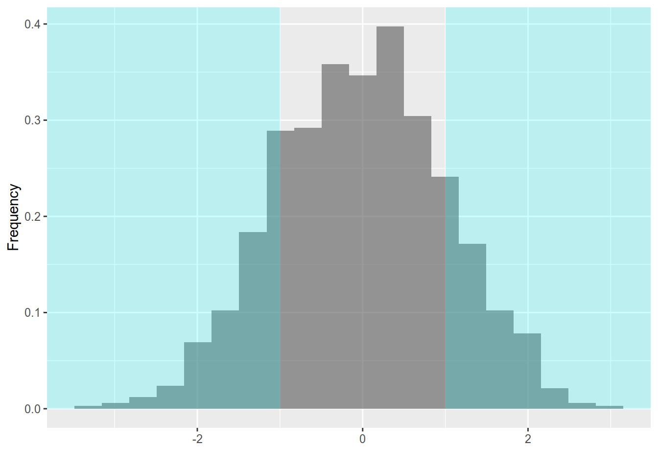
First we will use an arbitrarily constructed rejection region: \(RR = (-\infty, -1] \cup [1, \infty)\) and will examine the rate of wrong decisions that we make if we reject \(H_0\) when \(t \in RR\) using a simulation.
To visualise the problem let us look at the distribution of the t-statistic assuming that (6.6) is true. We generate 1000 samples of size \(n = 114\) from a N(8,4) distribution (note that this is exactly the distribution under \(H_0\)). For each sample we compute the t-statistic according to (6.1) and obtain 1000 realisation of the statistic (one for each simulated sample). The summary of all these 1000 values is shown in 6.1. The values of the statistic ranged from -3.480 to 2.828. The average value was close to 0 as expected.
| Min | Q25 | Mean | Median | Q75 | Max |
|---|---|---|---|---|---|
| -3.479711 | -0.7568795 | -0.0251816 | -0.0149223 | 0.689451 | 2.827728 |

Figure 6.2: Histogram of simulated t-statistics. The null hypothesis is rejected in samples with a t-statistic less than -1 or more than 1 . (shaded regions to the left and to the right).
The number of datasets where the null hypothesis was rejected because the t-statistic was greater than 1 was 160. In 167 datasets the t-statistic was less than -1 so the null hypothesis will be rejected there as well. Be sure to understand that all datasets are generated from one and the same distribution: \(N(8,4)\) and rejecting \(H_0\) is a wrong decision in all datasets. Overall we wrongly rejected the null hypothesis in 327 datasets (32.7 percent).
The court trial equivalent of a false rejection of the null hypothesis is to convict an innocent person. Just as courts strive to minimise the rate of erroneous convictions we would like to control this type of error. The convention is to adopt a rejection rule (region) that wrongly rejects \(H_0\) in no more that 5 percent of the cases (datasets).
\[\begin{align} P_{H_0}(T \in RR) = 0.05 \end{align}\] The suffix \({H_0}\) under the probability indicates that we are computing that probability for the distribution of \(T\) under the null hypothesis (i.e. assuming that it is true).
When working with real datasets we usually see only one of all possibles datasets (in the simulation we saw 1000 possible datasets) so we must work with assumptions. The distribution of the t-statistic shown in (6.5) can help us here. From Section 4.5 we know how to compute quantiles of the t-distribution and we can construct a rejection region such that if \(H_0\) is true, the probability of false rejection is 0.05. Let us call the left boundary of the rejection region the lower critical value and the upper boundary: upper critical value.
For a fixed false rejection probability \(\alpha\) we can set the lower critical value to \(t_{\alpha / 2}(n - 1)\), the \(\alpha/2\) quantile, and the upper critical value to \(t_{1 - \alpha / 2}(n - 1)\), the \(1 - \alpha / 2\) quantile. The rejection region is now \((-\infty, t_{\alpha / 2}(n - 1)] \cup [t_{1 - \alpha / 2}(n - 1), +\infty)\). Let us compute the probability that a t-statistic falls in that region under the null hypothesis.
\[\begin{align} P_{H_0}(T \in (-\infty, t_{\alpha / 2}] \cup [t_{1 - \alpha / 2}, +\infty)) & = P_{H_0}(T < t_{\alpha / 2}) + P_{H_0}(T > t_{1 - \alpha / 2}) \\ & = \alpha / 2 + \alpha / 2 = \alpha. \end{align}\]
To construct a rejection region with a false rejection probability of 0.05 we can simply choose \(\alpha = 0.05\). The critical values are then \(t_{0.025}(n - 1)\) and \(t_{0.975}(n - 1)\). The level \(\alpha\) is called the significance level of the test.
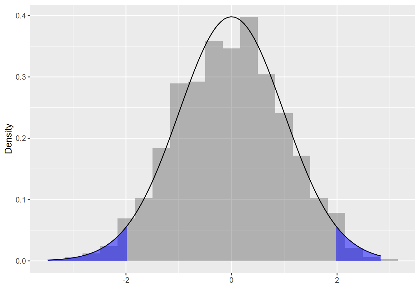
Figure 6.3 shows the rejection region for \(\alpha = 0.05\). The lower critical value is then \(t_{0.025}(114.00 - 1) = -1.981\) and the upper critical value is \(t_{0.975}(114.00 - 1) = 1.981\). The area under of the blue regions drawn over the intervals between the density of the t-distribution and the rejection region is 0.05, equal to the probability of the region.

Figure 6.3: Histogram of simulated t-statistics (under a true \(H_0\)). Overlayed is the density function of a \(t\)-distribution with \(n - 1\) degrees of freedom. The blue regions depict the area under the density of the t-distribution in the intervals \((-\infty, -1.981 )\) and \(( 1.98 , +\infty)\).
The number of datasets where the null hypothesis was rejected because the t-statistic was greater than 1.98 was 21. In 27 datasets the t-statistic was less than -1.98 so the null hypothesis was rejected there as well. Overall we wrongly rejected the null hypothesis in 48 datasets (4.8 percent) which is close to the expected rate of 5 percent (the significance level).
| lower | upper |
|---|---|
| -1.98118 | 1.98118 |
At a 5 percent significance level we reject the null hypothesis (\(H_0\)) in (6.6) that the expected incubation period is 8 days, because the value of the t-statistic (-6.135) is less that the lower critical value and thus lies inside the rejection region \((-\infty, -1.981] \cup [1.98 +\infty)\).
## $`Lower critical values`
##      0.01      0.05       0.1       0.2
## -2.626405 -1.984217 -1.660391 -1.290161
##
## $`Upper critival values`
##     0.01     0.05      0.1      0.2
## 2.626405 1.984217 1.660391 1.290161
##
## $`t-statistic`
## [1] 1.767767
6.3 p-value {sec:p-value}
In the previous section we showed how to construct rejection regions given a significance level \(\alpha\). The regions were two-sided, meaning that we rejected the null hypothesis for both too low and too high values of the t-statistic. Let us say that in a given sample we observe a value of the test-statistic equal to \(t\). The probability that we observe a value of the statistic \(T\) (the random variable) that is even more extreme than the observed value is called the p-value of the test. In the case of two-sided rejection regions more extreme means smaller than the observed for negative observed values and greater than the observed for positive values. Written more compactly this is:
\[\begin{align} P_{H_0}(|T| > |t|) \tag{6.7} \end{align}\]
At a significance level of 0.05 we reject \(H_0\) for p-values that are less than 0.05.
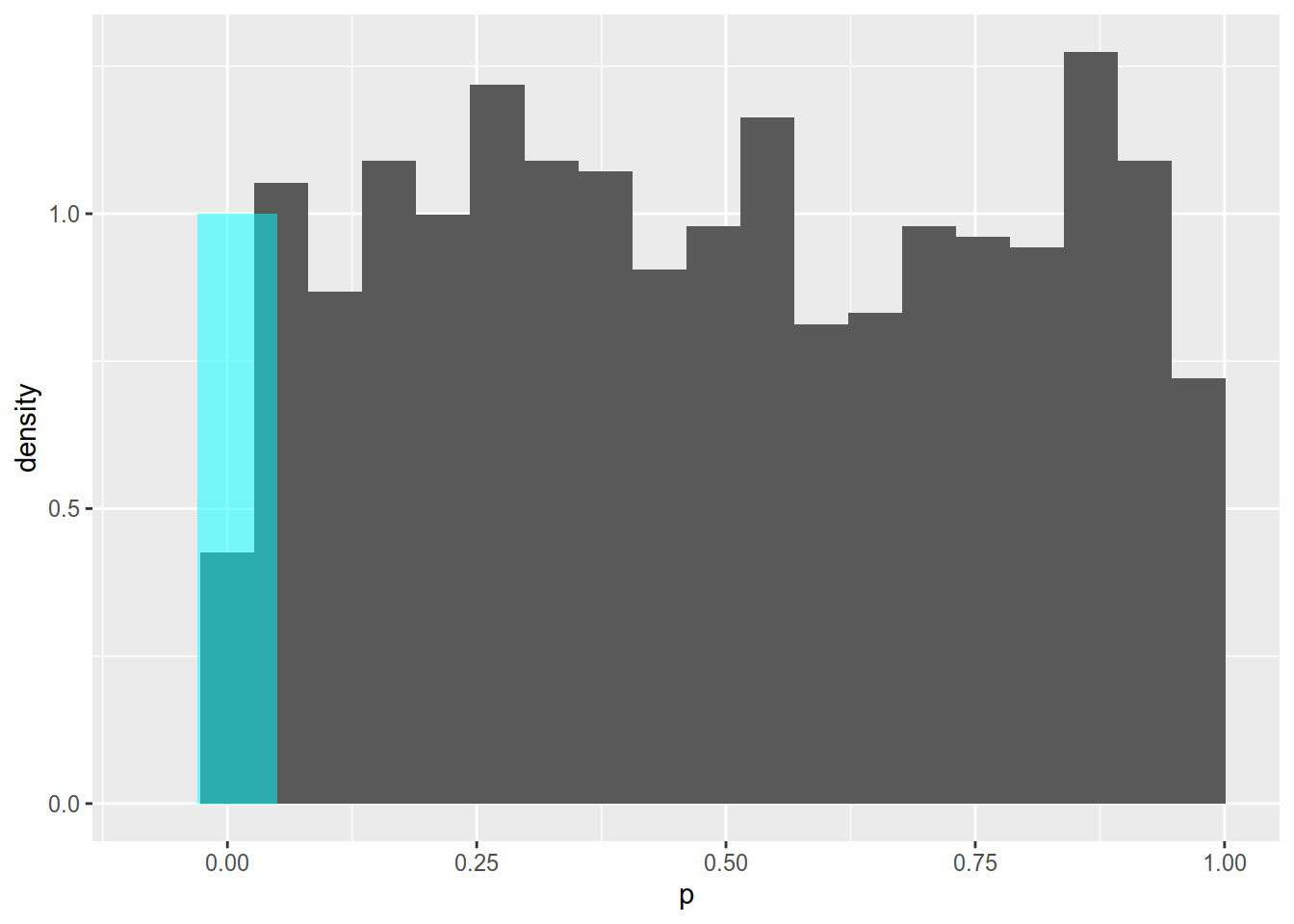
It is important to see that the p-value is a random variable, because it depends on \(T\). It can be shown that under the null hypothesis it follows a uniform distribution on the interval [0, 1] as you can see in Figure ?? which shows a histogram of 1000 t-test p-values generated from the null distribution (i.e. true null hypothesis).
## `summarise()` ungrouping output (override with `.groups` argument)## [1] 0.046
Figure 6.4: Histogram of p-values of a two-sided t-test for 1000 samples generated from the null distribution. The null hypothesis is rejected for p-values less than 0.05 (blue region).
Rejecting \(H_0\) for \(\text{p-value} < 0.05\) results in 46 out of 1000 false rejections (cyan segment of the histogram). This is close to the expected false rejection rate of 5 percent.
## [1] 0.02319784The probability to observe a value of \(T > 2.8\) or less than \(T < -2.8\) (more extreme than the observed value) is \[\begin{align} P_{t(8)}(T < -2.8 \cup T > 2.8) & = P_{t(8)}(T < -2.8) + P_{t(8)}(T > 2.8) \\ & = 2P_{t(8)}(T < -2.8) = \\ & = 0.02. \end{align}\] Here we use the fact that the t-distribution is symmetrical and therefore \(P_{t(8)}(T < -2.8) = P_{t(8)}(T > 2.8)\).
6.4 One-sided tests
Let us change the claim of the scientist from “The expected incubation period is exactly 8.00 days” to “The expected stay in hospital is greater than 8.00 days”. Now let us express the second statement in terms of \(\mu\):
\[\begin{align} H_0: \mu \geq \mu_0 = 8 \tag{6.8} \\ H_1: \mu < \mu_0 = 8 \end{align}\]
We will test this hypothesis with the same test statistic that we used in the two sided case but this time we will reject for small values of the statistic only, because large values of the statistic are consistent with \(H_0\). This type of hypothesis tests are called one-sided, because the rejection region is only one interval.
Let us reject the hypothesis for values of the t-statistic less than \(t_{0.05}(n - 1)\). The probability of false rejection of the null hypothesis is:
\[\begin{align} P_{H_0}(T < t_{0.05}) = 0.05 \end{align}\]
The value of the t-statistic is the same as in the two sided case: \(-6.13\). This time there is only one critical value: \(t_{0.05}(114 - 1) = -1.6584502\). The test statistic is less than the critical value, so we reject \(H_0\).
–>